library(tidyverse)
library(readxl)
library(sjPlot)HW 03: Data wrangling
Suggested Answers
Purpose
Real data rarely shows up ready to analyze. It comes in different file types, spread across more than one table, or shaped in a way that doesn’t match the plot you want to make. In this assignment you’ll import, recode, join, and reshape four small datasets.
- Import data from CSV and Excel files
- Create new variables with
case_when() - Join two data frames and reorder factor levels for a plot
- Reshape data with
pivot_wider()andpivot_longer()
Grading Rubric
- (2 pt) Commit history: on time and at least one commit per part I-IV.
- (4-5 pts ea.) Each part will be graded for correctness and completion.
While many of these steps could be combined into a single step using chaining methodology, please do the work clearly under the assigned question number. For example, don’t answer Question 8 as part of Q7, or Q5 as part of Q4.
Getting started
Load the tidyverse and readxl packages. All of the data for this assignment is in your data folder.
Part I. Age gaps in movies
The age-gaps.xlsx file lists couples in Hollywood movies and the ages of the two actors. The data is on the sheet called Hollywood Age Gaps, below 2 rows of notes.
1. Import from Excel
Read in age-gaps.xlsx with the appropriate read_ function and save it as a data frame named age_gaps. Starter code has been provided.
age_gaps <- read_excel(here::here("hw/data/age-gaps.xlsx"),
                       sheet = "Hollywood Age Gaps",
                       skip = 2)
head(age_gaps)
# A tibble: 6 × 13
movie_name release_year director age_difference couple_number actor_1_name
<chr> <dbl> <chr> <dbl> <dbl> <chr>
1 Harold and Ma… 1971 Hal Ash… 52 1 Ruth Gordon
2 Venus 2006 Roger M… 50 1 Peter O'Too…
3 The Quiet Ame… 2002 Phillip… 49 1 Michael Cai…
4 The Big Lebow… 1998 Joel Co… 45 1 David Huddl…
5 Beginners 2010 Mike Mi… 43 1 Christopher…
6 Poison Ivy 1992 Katt Sh… 42 1 Tom Skerritt
# ℹ 7 more variables: actor_2_name <chr>, character_1_gender <chr>,
# character_2_gender <chr>, actor_1_birthdate <chr>,
# actor_2_birthdate <dttm>, actor_1_age <dbl>, actor_2_age <dbl>2. Who is older?
Use filter to keep rows where the gender of character 1 and character 2 are not the same. Then use case_when() to create a new variable to identify which gender is older (regardless if the older person is character 1 or 2). Call this variable older and create values of "man older", "woman older", or "same age". Save the result as age_gaps_mw.
age_gaps_mw <- age_gaps |>
  filter(character_1_gender != character_2_gender) |>
  mutate(older = case_when(
    character_1_gender == "woman" & actor_1_age > actor_2_age ~ "woman older",
    character_2_gender == "woman" & actor_2_age > actor_1_age ~ "woman older",
    character_1_gender == "man" & actor_1_age > actor_2_age ~ "man older",
    character_2_gender == "man" & actor_2_age > actor_1_age ~ "man older",
    actor_1_age == actor_2_age ~ "same age"))
head(age_gaps_mw)
# A tibble: 6 × 14
movie_name release_year director age_difference couple_number actor_1_name
<chr> <dbl> <chr> <dbl> <dbl> <chr>
1 Harold and Ma… 1971 Hal Ash… 52 1 Ruth Gordon
2 Venus 2006 Roger M… 50 1 Peter O'Too…
3 The Quiet Ame… 2002 Phillip… 49 1 Michael Cai…
4 The Big Lebow… 1998 Joel Co… 45 1 David Huddl…
5 Poison Ivy 1992 Katt Sh… 42 1 Tom Skerritt
6 Whatever Works 2009 Woody A… 40 1 Larry David
# ℹ 8 more variables: actor_2_name <chr>, character_1_gender <chr>,
# character_2_gender <chr>, actor_1_birthdate <chr>,
# actor_2_birthdate <dttm>, actor_1_age <dbl>, actor_2_age <dbl>, older <chr>3. Plot who is older
Make a bar plot of older. What do you notice?
plot_frq(age_gaps_mw$older) +
  labs(x = NULL, y = "Number of couples",
       title = "Who is older in Hollywood couples?")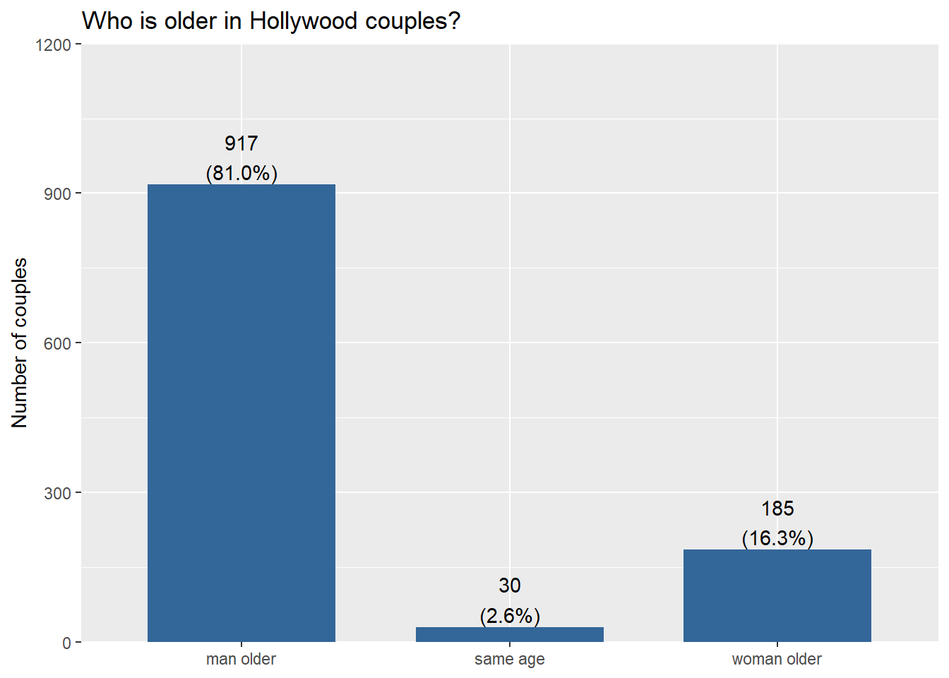
The man is older in most couples the vast majority of the time (80%). Couples where the woman is older are much less common, and same-age couples are rare.
Part II. Sales taxes by region
This part uses the following two data sets:
sales-taxes-25.csvhas 2025 state and local sales tax rates for each state.us-regions.csvlists the Census region for each state.
4. Import two files
Read in both data sets and save them as sales_taxes and us_regions.
sales_taxes <- read_csv(here::here("hw/data/sales-taxes-25.csv"))
us_regions <- read_csv(here::here("hw/data/us-regions.csv"))
head(sales_taxes)
# A tibble: 6 × 7
state state_tax_rate state_tax_rank avg_local_tax_rate max_local
<chr> <dbl> <dbl> <dbl> <dbl>
1 Alabama 4 40 5.44 11
2 Alaska 0 46 1.82 7.85
3 Arizona 5.6 28 2.92 5.3
4 Arkansas 6.5 9 2.98 6.12
5 California 7.25 1 1.73 5.25
6 Colorado 2.9 45 4.96 8.3
# ℹ 2 more variables: combined_tax_rate <dbl>, combined_rank <dbl>head(us_regions)# A tibble: 6 × 2
state_name region
<chr> <chr>
1 Maine Northeast
2 New Hampshire Northeast
3 Vermont Northeast
4 Massachusetts Northeast
5 Rhode Island Northeast
6 Connecticut Northeast5. Join
Use left_join() to add each state’s region to sales_taxes. The state name is called state in one data frame and state_name in the other, so use join_by(state == state_name). Save the result as taxes_regions.
taxes_regions <- sales_taxes |>
  left_join(us_regions, join_by(state == state_name))
head(taxes_regions)
# A tibble: 6 × 8
state state_tax_rate state_tax_rank avg_local_tax_rate max_local
<chr> <dbl> <dbl> <dbl> <dbl>
1 Alabama 4 40 5.44 11
2 Alaska 0 46 1.82 7.85
3 Arizona 5.6 28 2.92 5.3
4 Arkansas 6.5 9 2.98 6.12
5 California 7.25 1 1.73 5.25
6 Colorado 2.9 45 4.96 8.3
# ℹ 3 more variables: combined_tax_rate <dbl>, combined_rank <dbl>,
# region <chr>6. Tax rates by region
6a. Reorder
Use fct_reorder() to order region by combined_tax_rate. Save the result back to taxes_regions.
taxes_regions <- taxes_regions |>
  mutate(region = fct_reorder(region, combined_tax_rate))
head(taxes_regions)
# A tibble: 6 × 8
state state_tax_rate state_tax_rank avg_local_tax_rate max_local
<chr> <dbl> <dbl> <dbl> <dbl>
1 Alabama 4 40 5.44 11
2 Alaska 0 46 1.82 7.85
3 Arizona 5.6 28 2.92 5.3
4 Arkansas 6.5 9 2.98 6.12
5 California 7.25 1 1.73 5.25
6 Colorado 2.9 45 4.96 8.3
# ℹ 3 more variables: combined_tax_rate <dbl>, combined_rank <dbl>,
# region <fct>6b. Boxplot
Make a boxplot of combined_tax_rate for each region. What do you notice? Why is there a NA in the plot?
ggplot(taxes_regions, aes(x = combined_tax_rate, y = region)) +
  geom_boxplot() +
  labs(x = "Combined state and local sales tax rate (%)", y = NULL,
       title = "Sales tax rates by region")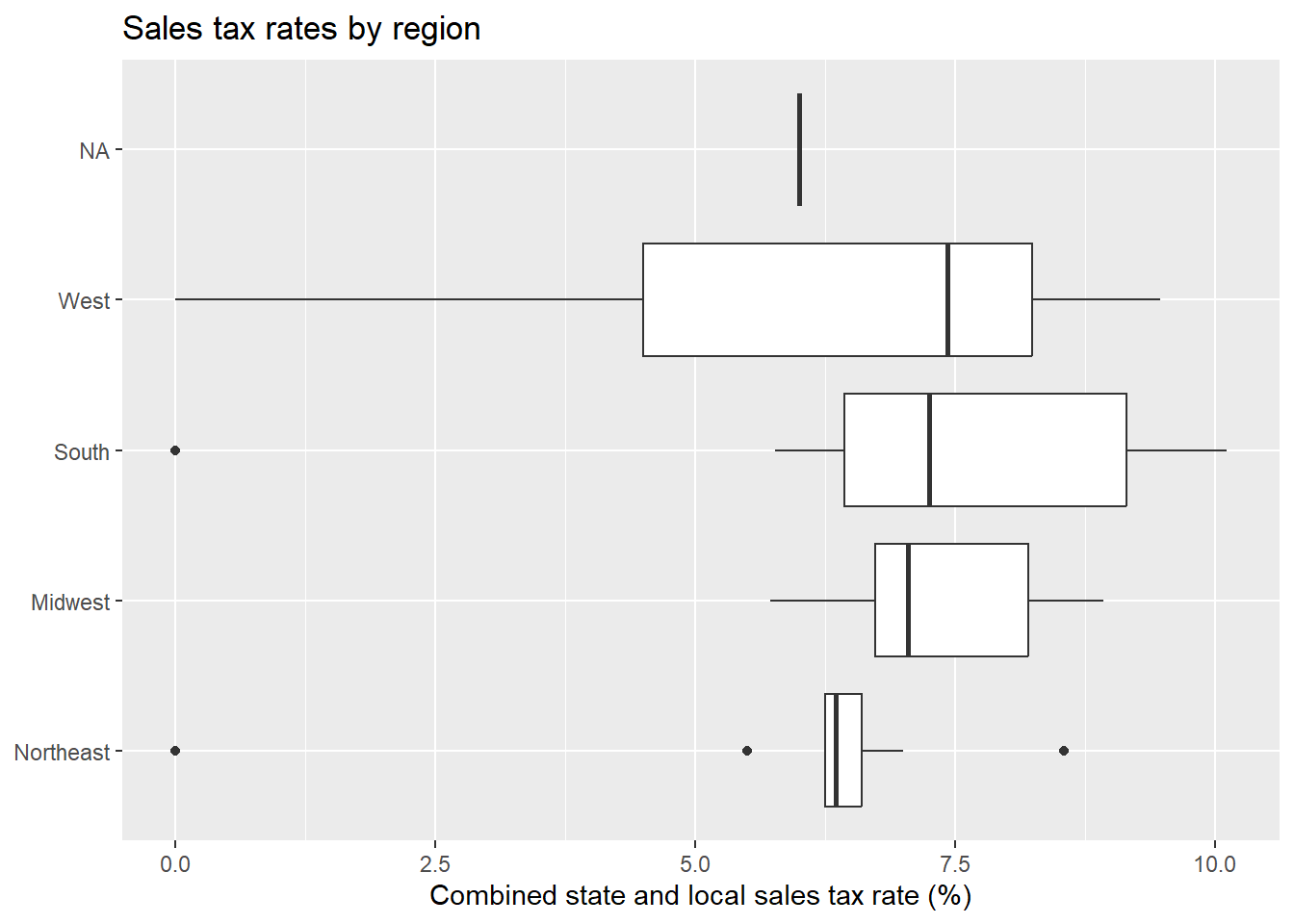
The West has the highest median combined rate, just above the South. The Northeast has the lowest. The NA box is Washington, DC, which isn’t in us_regions.
Part III. Minimum wage and employment
On April 1, 1992, New Jersey raised its minimum wage from $4.25 to $5.05 per hour. Pennsylvania did not. Economists David Card and Alan Krueger surveyed fast-food restaurants on both sides of the border before and after the change to see whether the higher wage cost jobs. Here are some variable definitions.
id: restaurant IDstate:NJorPAtime:beforeorafterthe wage increasewage: starting wage in dollarsfte: full-time-equivalent employees (full-time workers plus half the part-time workers)
7. Import and pivot wider
Read in card-krueger.csv. Then use pivot_wider() to create card_krueger_wide with one row per restaurant and the columns id, state, wage_before, wage_after, fte_before, and fte_after.
card_krueger_wide <- read_csv(here::here("hw/data/card-krueger.csv")) |>
  pivot_wider(names_from = time, values_from = c(wage, fte))
head(card_krueger_wide)
# A tibble: 6 × 6
id state wage_before wage_after fte_before fte_after
<dbl> <chr> <dbl> <dbl> <dbl> <dbl>
1 46 PA NA 4.3 40.5 24
2 49 PA NA 4.45 13.8 11.5
3 506 PA NA 5 8.5 10.5
4 56 PA 5 5.25 34 20
5 61 PA 5.5 4.75 24 35.5
6 62 PA 5 NA 20.5 NA 8. Change in employment
Add a new variable called fte_change that equals fte_after - fte_before.
card_krueger_wide <- card_krueger_wide |>
  mutate(fte_change = fte_after - fte_before)
head(card_krueger_wide)
# A tibble: 6 × 7
id state wage_before wage_after fte_before fte_after fte_change
<dbl> <chr> <dbl> <dbl> <dbl> <dbl> <dbl>
1 46 PA NA 4.3 40.5 24 -16.5
2 49 PA NA 4.45 13.8 11.5 -2.25
3 506 PA NA 5 8.5 10.5 2
4 56 PA 5 5.25 34 20 -14
5 61 PA 5.5 4.75 24 35.5 11.5
6 62 PA 5 NA 20.5 NA NA 9. Compare states
Use group_by() and summarize() to find the mean fte_change in each state. Did employment fall in New Jersey after the wage increase?
card_krueger_wide |>
  group_by(state) |>
  summarize(mean_fte_change = mean(fte_change, na.rm = TRUE))
# A tibble: 2 × 2
state mean_fte_change
<chr> <dbl>
1 NJ 0.467
2 PA -2.28 No. Employment rose slightly in New Jersey (about +0.5 FTE per restaurant) and fell in Pennsylvania (about −2.3). This is the opposite of what the simple “higher wages cost jobs” story predicts.
Part IV. Income distribution
The acs5_income.csv file was downloaded directly from the U.S. Census Bureau. It shows the percent of households in each income bracket for every county in California.
Each row is an income bracket. Each column is one county, for one household type (households, families, married-couple families, or nonfamily households), for either the estimate or its margin of error. That’s 465 columns!
10. Import
Read in acs5_income.csv. Keep only the first column and the estimate columns for all households, and save the result as acs_income. Variables can be renamed on the fly in the select statement using select(newname = oldname), and the helper function contains("!!Households!!Estimate") will select every column with that literal text in its name.
acs_income <- read_csv(here::here("hw/data/acs5_income.csv")) |>
  select(income = `Label (Grouping)`, contains("!!Households!!Estimate"))
head(acs_income)
# A tibble: 6 × 59
income Alameda County, Cali…¹ Alpine County, Calif…² Amador County, Calif…³
<chr> <chr> <chr> <chr>
1 Total 593,117 473 16,066
2 Less… 4.00% 2.30% 5.90%
3 $10,… 2.70% 2.10% 3.30%
4 $15,… 4.10% 4.00% 3.90%
5 $25,… 3.90% 8.20% 6.10%
6 $35,… 6.30% 5.50% 9.30%
# ℹ abbreviated names: ¹`Alameda County, California!!Households!!Estimate`,
# ²`Alpine County, California!!Households!!Estimate`,
# ³`Amador County, California!!Households!!Estimate`
# ℹ 55 more variables: `Butte County, California!!Households!!Estimate` <chr>,
# `Calaveras County, California!!Households!!Estimate` <chr>,
# `Colusa County, California!!Households!!Estimate` <chr>,
# `Contra Costa County, California!!Households!!Estimate` <chr>, …11. Pivot longer
Filter out the total row, then use pivot_longer() on every column except income, with the column names in county and the values in percent. Save the result as income_long.
income_long <- acs_income |>
  filter(income != "Total") |>
  pivot_longer(-income, names_to = "county", values_to = "percent")
head(income_long)
# A tibble: 6 × 3
income county percent
<chr> <chr> <chr>
1 Less than $10,000 Alameda County, California!!Households!!Estimate 4.00%
2 Less than $10,000 Alpine County, California!!Households!!Estimate 2.30%
3 Less than $10,000 Amador County, California!!Households!!Estimate 5.90%
4 Less than $10,000 Butte County, California!!Households!!Estimate 6.00%
5 Less than $10,000 Calaveras County, California!!Households!!Estim… 5.00%
6 Less than $10,000 Colusa County, California!!Households!!Estimate 5.60% 12. Clean up
percent was read in as text because the values have % signs, and every county name ends in the same long piece of text. Use parse_number() to drop everything that isn’t part of a number, and str_remove() to delete a piece of text. Lastly filter to only keep 4 counties of your choice to compare to Butte (that is, choose Butte county and 4 others.)
Starter code has been provided for you.
income_long <- income_long |>
  mutate(percent = parse_number(percent),
         county = str_remove(county,
                             " County, California!!Households!!Estimate")) |>
    filter(county %in% c("Butte", "Tehama", "Glenn", "Plumas", "Yuba"))
head(income_long)
# A tibble: 6 × 3
income county percent
<chr> <chr> <dbl>
1 Less than $10,000 Butte 6
2 Less than $10,000 Glenn 3.5
3 Less than $10,000 Plumas 5.3
4 Less than $10,000 Tehama 5.2
5 Less than $10,000 Yuba 6.1
6 $10,000 to $14,999 Butte 4 13. Income by county
Make a bar plot with one bar per county, filled by income bracket. Refer back to wk6-d03 (Recoding data) and use the income by religion plot at the end of it as a guide. Where does Butte County fall compared with your chosen 4 counties?
When you create the plot, confirm the income brackets are in the order you expect.
income_long |>
  mutate(income = fct_inorder(income)) |>
  ggplot(aes(x = percent, y = county, fill = income)) +
  geom_col(position = "fill") +
  scale_fill_viridis_d() +
  theme_minimal() +
  theme(legend.position = "bottom") +
  guides(fill = guide_legend(nrow = 3, byrow = TRUE)) +
  labs(x = "Proportion", y = "",
       title = "Household income distribution by California county, 2019-2023",
       subtitle = "Source: U.S. Census Bureau, ACS 5-year estimates, Table S1901",
       fill = "Income")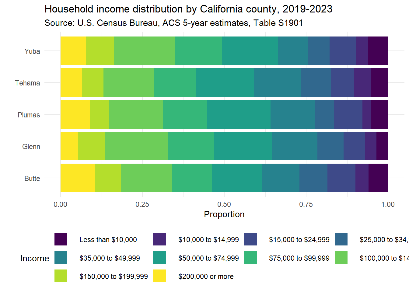
Butte County has a pretty even distribution of income brackets, with the highest amount of household incomes over $200,000, and comparable proportions of $25k and under to other counties. Glenn and Yuba have the higher proportion of households between $100 and $150k. > Note: I was able to use fct_inorder here to display the income categories in order in which they appeared in the data set. This only works because they were already in order, and i didn’t do any sorting/rearranging. This is a fragile approach. If I thought that there was the potential to get new, unordered data or sorting done ahead of time I would use other functions like fct_relevel.
Note
This page uses data and ideas from STA 199, Fall 2025 by Mine Çetinkaya-Rundel (AE 06: sales taxes, AE 08: age gaps, HW 4: Card and Krueger minimum wage data). Modified: new questions combining four datasets for data import, recoding, joins, factors, and pivoting.
Data citation: U.S. Census Bureau, U.S. Department of Commerce. “Income in the Past 12 Months (in 2023 Inflation-Adjusted Dollars).” American Community Survey, ACS 5-Year Estimates Subject Tables, Table S1901, https://data.census.gov/table/ACSST5Y2023.S1901?t=Income+and+Poverty&g=040XX00US06$0500000. Accessed on 27 Sep 2026.