library(tidyverse);library(gtsummary)
library(sjPlot);library(ggpubr)

airbnb <- read_csv(here::here("hw/data/listings.csv")) |>
  mutate(price = parse_number(price),
         superhost = factor(host_is_superhost,
labels = c("Not a superhost", "Superhost")))Describing distributions and relationships
A writing guide
Purpose
You know how to write the code to make a plot and a table of summary statistics. This guide is about the next part: describing in words what they show. Communication of your findings is a critical part to being a good Data Scientist. Any time an assignment says describe, compare or interpret, refer to these guidelines.
The examples use the San Francisco Airbnb listings from hw02. Each one has a plot, summary statistics, and then an example paragraph. Since I am demonstrating quality writing, I am going to use plotting functions from the ggpubr and sjPlot package to also demonstrate quality plots.
The three-part recipe
Every description needs three things:
- A plot, with a title and axis labels that include units.
- Summary statistics.
- A few sentences that connect the numbers to the plot, in plain English, with units and context.
Note
Plots should never stand alone. They should always be accompanied by a sentence that describes the features of the plot, along with the summary numbers to put the data in context.
For a single variable it looks like this:
| Quantitative variable | Categorical variable | |
|---|---|---|
| Plot | histogram and boxplot | bar chart (plot_frq()) |
| Summary statistics | n, min, Q1, median, mean, Q3, max, SD, IQR | count and percent for each category |
| Sentences | center, shape, spread, unusual values | N and % for the largest category, plus anything that shouldn’t be there |
Describing one variable
Quantitative variables
📖 Reading: IMS 5.3 Histograms and shape, IMS 5.6 Robust statistics, R4DS 10.3 Variation
Cover these four things:
- Center: What’s a typical value? Use the median if the data are skewed or have outliers. Use the mean if they’re roughly symmetric.
- Shape: Symmetric or skewed? One peak or more than one? The reading above explains the vocabulary.
- Spread: How much do the values vary? The median goes with the IQR, the mean goes with the SD. Give the min and max too.
- Unusual values: Outliers, impossible values, a pile-up at one number. Say what they are and what you did about them.
Example: review rating
review_scores_rating is the overall rating guests gave the listing, from 1 to 5.
gghistogram(airbnb$review_scores_rating, add = "mean", binwidth = 0.25)+
  labs(x = "Review score rating", y = "Count", title = "Distribution of review scores")
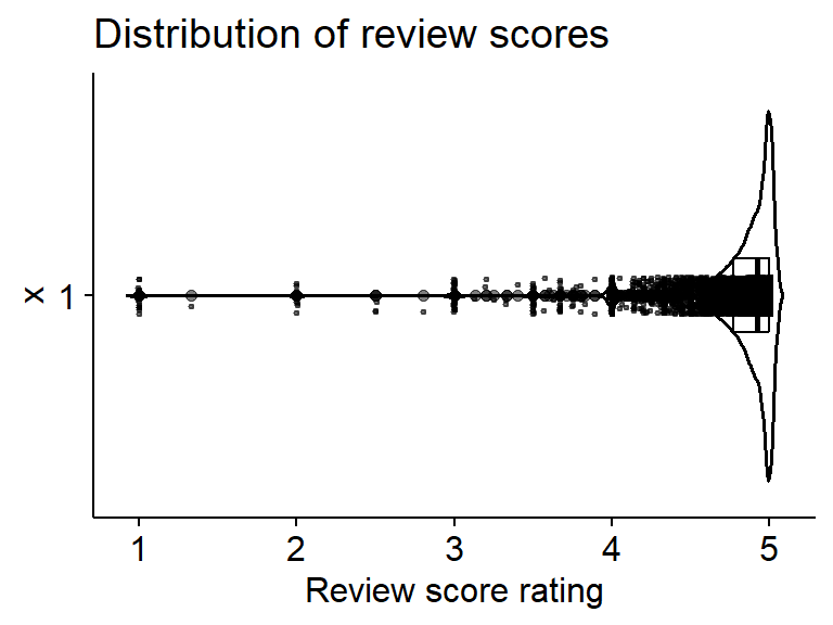
ggviolin(airbnb$review_scores_rating, add = c("jitter", "boxplot"),
         add.params = list(jitter = 0.05, alpha = .5, size = .5)) + coord_flip() +
  labs(y = "Review score rating", title = "Distribution of review scores")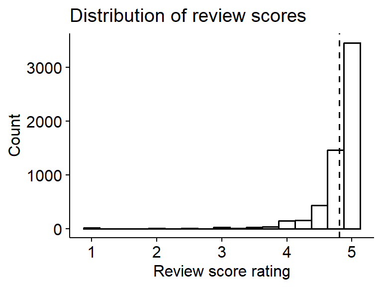
summary(airbnb$review_scores_rating) Min. 1st Qu. Median Mean 3rd Qu. Max. NAs
1.000 4.770 4.920 4.803 5.000 5.000 1584 sd(airbnb$review_scores_rating, na.rm = TRUE)[1] 0.3676205Categorical variables
📖 Reading: IMS 4.1 Contingency tables and bar plots, R4DS 1.4.1 A categorical variable
Cover these things:
- What the categories are.
- N and % for at least the largest category. The count by itself doesn’t tell me how common it is, and the percent by itself doesn’t tell me how much data it’s based on.
- The smaller categories, if they matter.
- Any category that shouldn’t be there (e.g. “Undefined”, “Other”, a typo).
For a binary variable you only need to describe one of the categories, since the other one is 100% minus that.
Example: room type
plot_frq(airbnb$room_type) + ylim(c(0, 5500)) + labs(x = "Room Type")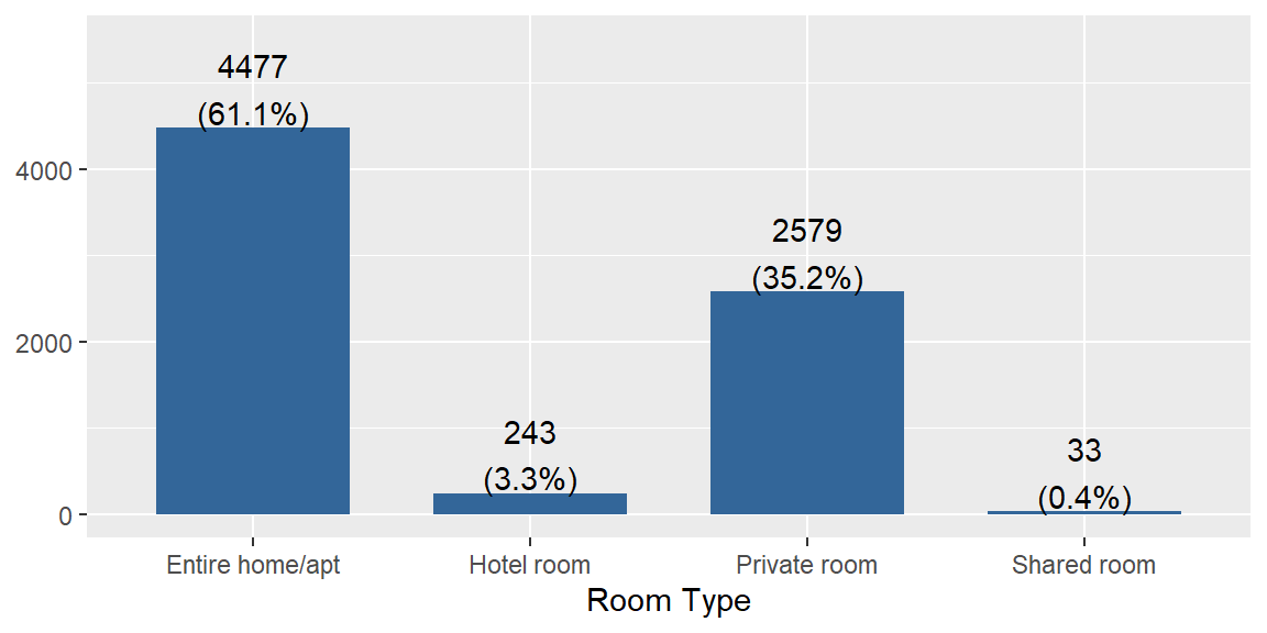
Binary example: superhost.
tbl_summary(airbnb, include = "superhost",
digits = all_categorical() ~ c(0, 1))| Characteristic | N = 7,3321 |
|---|---|
| superhost | |
| Not a superhost | 3,817 (52.7%) |
| Superhost | 3,425 (47.3%) |
| Unknown | 90 |
| 1 n (%) | |
Describing a relationship
Before you plot anything, decide which variable is the explanatory variable (the one you think helps explain things, usually the x-axis) and which is the response (the outcome, usually the y-axis). In the Airbnb data a couple of natural questions are what goes along with the price of a listing, and what goes along with the host being a superhost.
The right plot and summary depend on the types of the two variables. A binary variable counts as categorical with two levels.
| Response ~ Explanatory | Plot | Summary statistics | Sentences |
|---|---|---|---|
| C ~ C | side by side bars with row percents (plot_xtab()) |
counts and percents within each group (tbl_summary(by = )) |
the % in the response category for each explanatory category, and the difference in percentage points |
| Q ~ C | faceted histograms (gghistogram(facet.by = )) or violin plots with boxplots (ggviolin()) |
grouped summarise() |
center, shape and spread for each group |
| Q ~ Q | scatterplot with a smooth line | correlation, cor() |
direction, strength and form |
Note
Use numbers and comparison words. Say “higher” or “more spread out”, and then say by how much (higher by $120, a difference of 7.5 percentage points).
Categorical response, categorical explanatory (C ~ C)
📖 Reading: IMS 4.2 Visualizing two categorical variables, IMS 4.3 Row and column proportions, R4DS 10.5.2 Two categorical variables
Looking at counts only gives you half the story. Groups of different sizes can’t be fairly compared with counts, so compare the percents within each group of the explanatory variable (row percents). Put the explanatory variable in by = for tbl_summary(), and first in plot_xtab().
Example: room type and superhost
Is the type of room related to whether the host is a superhost? Room type is the explanatory variable and superhost is the response. Each column of the table is one room type, so the percents add up to 100% within each room type. tbl_summary() leaves the listings with no superhost value out of the percents, and counts them in the Unknown row.
tbl_summary(airbnb, by = room_type, include = superhost,
digits = all_categorical() ~ c(0, 1))| Characteristic | Entire home/apt N = 4,4771 |
Hotel room N = 2431 |
Private room N = 2,5791 |
Shared room N = 331 |
|---|---|---|---|---|
| superhost | ||||
| Not a superhost | 2,161 (48.3%) | 238 (97.9%) | 1,389 (55.8%) | 29 (87.9%) |
| Superhost | 2,316 (51.7%) | 5 (2.1%) | 1,100 (44.2%) | 4 (12.1%) |
| Unknown | 0 | 0 | 90 | 0 |
| 1 n (%) | ||||
plot_xtab(x = airbnb$room_type, grp = airbnb$superhost,
          show.total = FALSE, margin = "row") + labs(x = "Room Type")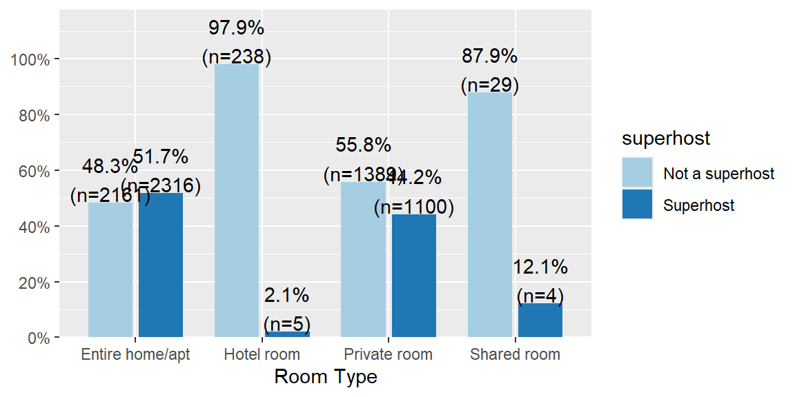
Quantitative response, categorical explanatory (Q ~ C)
📖 Reading: IMS 4.6 Comparing numerical data across groups, R4DS 10.5.1 A categorical and a numerical variable
Describe the center, shape and spread within each group, and use comparison words with numbers.
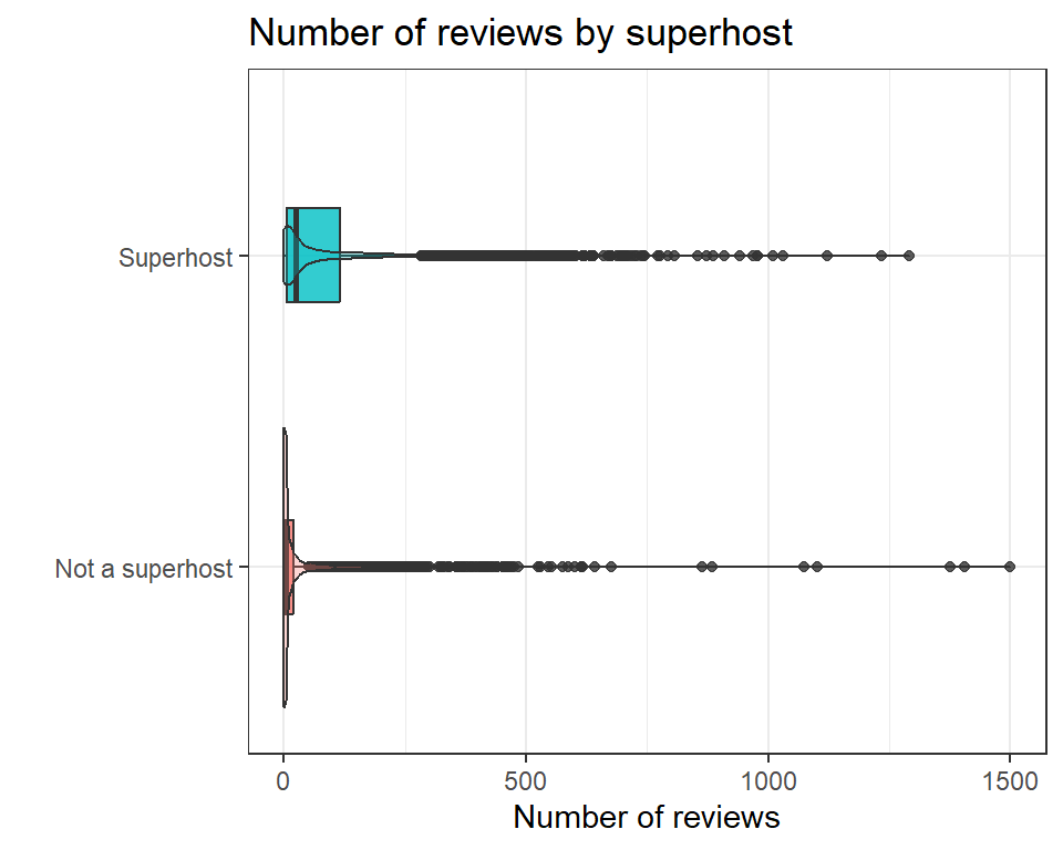
Example: number of reviews by superhost
Do superhosts get more reviews? Superhost is the explanatory variable and the number of reviews (number_of_reviews) is the response. I’m dropping the 90 listings with no superhost value so every listing is in one of the two groups.
airbnb_sh <- airbnb |> drop_na(superhost)

gghistogram(airbnb_sh, x = "number_of_reviews", binwidth = 25, fill = "superhost", facet.by = "superhost") +
  labs(x = "Number of reviews", y = "Count", title = "Number of reviews by superhost")
ggplot(airbnb_sh, aes(x = superhost, y = number_of_reviews, fill = superhost)) +
  geom_boxplot(width = .3, alpha = .8) + geom_violin(alpha = .3) +
  labs(x = "", y = "Number of reviews", title = "Number of reviews by superhost") + theme_bw() +
  coord_flip() + theme(legend.position = "none")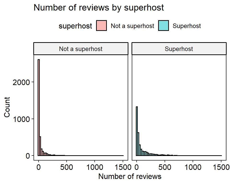
airbnb_sh |>
  group_by(superhost) |>
  summarise(
    n = n(),
    min = min(number_of_reviews),
    q1 = quantile(number_of_reviews, 0.25),
    median = median(number_of_reviews),
    mean = mean(number_of_reviews),
    sd = sd(number_of_reviews),
    iqr = IQR(number_of_reviews),
    max = max(number_of_reviews)
  )
# A tibble: 2 × 9
superhost n min q1 median mean sd iqr max
<fct> <int> <dbl> <dbl> <dbl> <dbl> <dbl> <dbl> <dbl>
1 Not a superhost 3817 0 0 3 31.2 86.1 20 1500
2 Superhost 3425 0 5 24 91.5 149. 111 1292Quantitative response, quantitative explanatory (Q ~ Q)
📖 Reading: IMS 5.1 Scatterplots for paired data, IMS 7.1.4 Describing linear relationships with correlation, R4DS 10.5.3 Two numerical variables
A scatterplot is the main tool. Describe three things:
- Direction: Is the association positive or negative?
- Strength: Is the relationship strong or weak? The correlation coefficient r helps here, but only for straight-line patterns.
- Form: Is it linear? Curved? Clumped into clusters? Any outliers?
Important
The correlation only measures how well the points follow a straight line. That’s why you always have to look at the plot and not just report r.
Example: number of guests and price
How many people a listing sleeps (accommodates) is the explanatory variable and price is the response. Like in hw02, I’m only using listings priced at $1000 or less (airbnb_1k). That leaves out the 384 listings priced above $1000, and the 1,400 listings with no price.
There are thousands of points, so they pile on top of each other. Making them see-through (alpha) lets the crowded spots show up darker. The curvy line is a smooth trend and the red line is the best straight line.
airbnb_1k <- airbnb |> filter(price <= 1000)

ggplot(airbnb_1k, aes(x = accommodates, y = price)) +
  geom_point(alpha = 0.3) +
  geom_smooth(se = FALSE) +
  geom_smooth(method = "lm", se = FALSE, color = "red") +
  labs(x = "Number of guests the listing sleeps", y = "Price ($)",
       title = "Price by number of guests")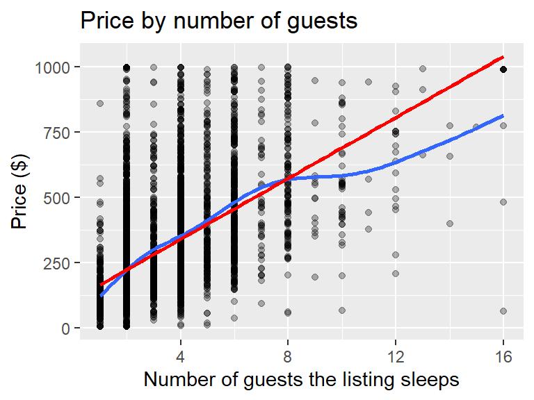
cor(airbnb_1k$accommodates, airbnb_1k$price)[1] 0.5502468Sentence templates
These are just a starting point. Fill in the brackets, then wordsmith it so that it sounds more natural and somewhat like you wrote it. This is a spot where the more you practice writing the better you will get, but we all start by copying good examples then making it our own.
One quantitative variable
The distribution of [variable] is [symmetric / right skewed / left skewed]. The median [variable] is [value] [units] and half of the values are between [Q1] and [Q3] (IQR = [value]). Values range from [min] to [max]. [Anything unusual, and what you did about it.]
One categorical variable
The most common [variable] is [category] at [percent]% (n = [N]). [Next biggest categories.] [Anything unusual, like tiny categories or categories that shouldn’t be there.]
Categorical response ~ categorical explanatory
[Percent]% (n = [N]) of [group A] [response], compared with [percent]% (n = [N]) of [group B], a difference of [X] percentage points. [Anything surprising, or any group that is really small.]
Quantitative response ~ categorical explanatory
[Group A] tends to have [higher / lower] [variable] than [group B], with a median of [value] compared with [value]. [Group A] is [more / less] spread out (SD = [value] compared with [value]). [Shape of each group and any outliers.]
Quantitative response ~ quantitative explanatory
There is a [negligible / weak / moderate / strong / very strong] [positive / negative] association between [x] and [y] (r = [value]). The relationship is [linear / curved / clumped]. [Any outliers, or any place the pattern changes.]