library(tidyverse)HW 02: EDA (key)
Suggested answers
Important
These are suggested answers. This document is a reference, not an exhaustive key.
Purpose
Airbnb has grown quickly in San Francisco, and its effect on the local housing market has become a real point of discussion. The website Inside Airbnb states that it is a “mission driven project that provides data and advocacy about Airbnb’s impact on residential communities.”
In this assignment we’ll explore a dataset of San Francisco Airbnb listings collected by Inside Airbnb to see how price and listing characteristics vary across room types.
- Practice translating a research question into a
dplyr/ggplot2pipeline - Choose an appropriate visualization for comparing a distribution across groups
- Use both a plot and summary statistics together to support a data-driven claim
Getting started
Load the tidyverse package. The data comes from Inside Airbnb as a compressed CSV file. You can learn more about the variables in the Inside Airbnb data dictionary.
Read in the San Francisco listings data. The price variable is stored with dollar signs and commas, so parse_number() converts it to a numeric variable that R can summarize and plot.
airbnb <- read_csv(
  "https://data.insideairbnb.com/united-states/ca/san-francisco/2026-06-14/data/listings.csv.gz"
) |>
  mutate(price = parse_number(price))
Important
The cache: true option tells Quarto to save the result of this code chunk after it runs. The next time you render the document, Quarto can reuse the saved result instead of downloading the Airbnb data again. If you change the code in this chunk or clear the cache, Quarto will run the chunk again.
Because the cache may contain downloaded data, add the /cache folder to your .gitignore file so the data is not pushed to GitHub.
Get familiar with the data before diving into the exercises. Use functions like glimpse() or str() and review the Inside Airbnb data dictionary to learn what each variable means.
# glimpse(airbnb)When you’re happy with your answers, commit and push your work to GitHub with a meaningful commit message.
Exercises
1. How many listings?
How many observations (rows) does the dataset have? Answer using inline code rather than hard-coding the number.
The dataset has 7332 listings.
2. What does a row represent?
Based on the data documentation and after looking at the data, what does each row in the dataset represent?
Each row represents a single Airbnb listing in San Francisco – one row per place that can be booked, not one row per host or per booking.
3. Price distribution
3a. Initial plot
Create a histogram and a boxplot that show the distribution of Airbnb prices. What do you notice about the shape of the distribution? Are there any values that seem extreme?
ggplot(airbnb, aes(x = price)) +
  geom_histogram(binwidth = 100) +
  labs(x = "Price", y = "Count",
       title = "Distribution of Airbnb listing price")
ggplot(airbnb, aes(x = price)) +
  geom_boxplot() +
  labs(x = "Price", y = "Count",
       title = "Distribution of Airbnb listing price")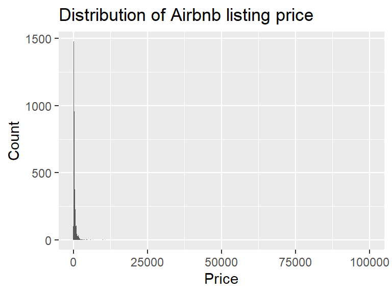
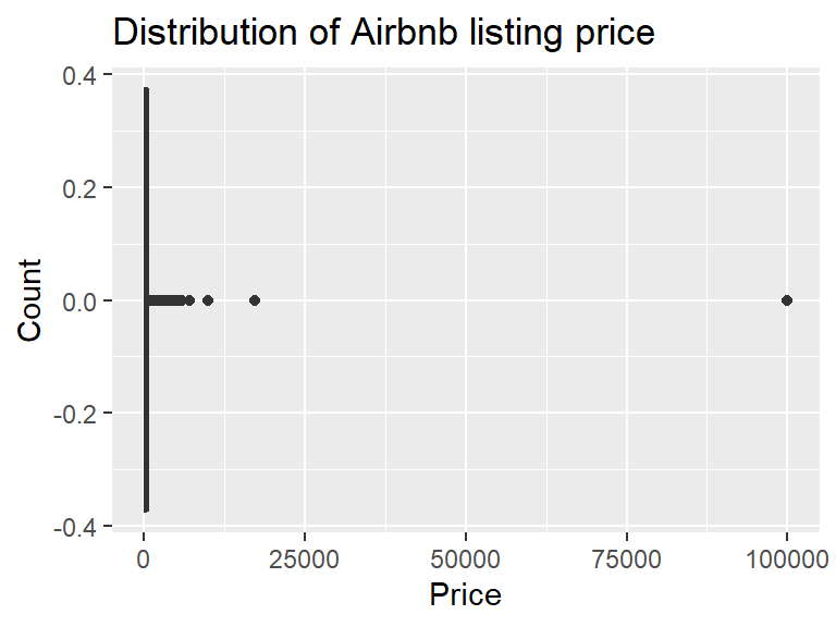
The distribution of Airbnb listing prices is strongly right skewed. Almost all of the listings are bunched up in the first few bars at the left, and a small number of listings with extremely high prices stretch the x-axis out. There are actually only a handful of listings above $10,000, and just one way out near $100,000. This squishes the boxplot into a thin line with a long string of outliers off to the right.
3b. Zoom in
Adjust your plots above to control the x-limits to only show prices below 5000. Comment on this new view.
ggplot(airbnb, aes(x = price)) +
  geom_histogram(binwidth = 100) +
  xlim(c(0,5000)) +
  labs(x = "Price", y = "Count",
       title = "Distribution of Airbnb listing price")
ggplot(airbnb, aes(x = price)) +
  geom_boxplot() +
  xlim(c(0,5000)) +
  labs(x = "Price", y = "Count",
       title = "Distribution of Airbnb listing price")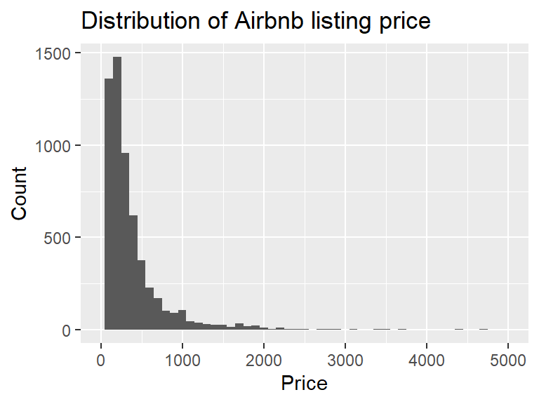
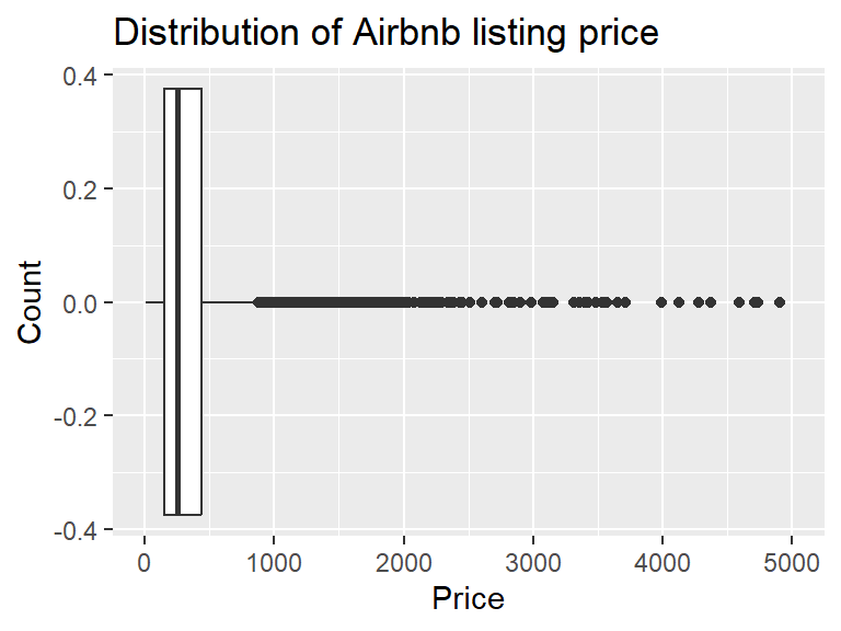
With the x-axis limited to prices below $5,000 the distribution is still strongly right skewed, but now we can actually see its shape. The bulk of the listings are priced below $1,000, with the tallest bars at the low end, and a long thin tail of listings between $1,000 and $5,000 that keeps trailing off. The boxplot still has a long string of high-priced outliers, so even in this zoomed in view the top of the price range is stretched out.
4. Summary statistics for price
Calculate the minimum, mean, median, standard deviation, IQR and maximum listing price. Interpret each number in context of the data set. Compare the mean and median - what does this tell you about the skew of the distribution? Based on this answer, which is the most appropriate measure of center? The mean or the median?
airbnb |>
  summarise(
    min = min(price, na.rm = TRUE),
    mean = mean(price, na.rm = TRUE),
    median = median(price, na.rm = TRUE),
    sd = sd(price, na.rm = TRUE),
    iqr = IQR(price, na.rm = TRUE),
    max = max(price, na.rm = TRUE)
  )
# A tibble: 1 × 6
min mean median sd iqr max
<dbl> <dbl> <dbl> <dbl> <dbl> <dbl>
1 4.14 414. 252. 1432. 287. 99999Prices for Airbnb listings range from $4.14 to $99,999, and both ends look implausible. The max is an odd number and MUCH larger than a typical listing price (the next highest is $17,308), and $4.14 for a night isn’t believable either. The mean price is $414, nearly double the median of $252, which confirms the strong right skew. Because the extreme prices pull the mean up, the median is the better measure of center. The standard deviation is huge at $1,432, again because of the extreme values, but the IQR is much smaller at $287, meaning the middle 50% of listings are priced within a $287 range of each other. With data this skewed the median and IQR describe a typical listing much better than the mean and SD.
5. Filtered summary statistics for price
Apply a filter to the airbnb data to keep only listings with prices at or below $1000. Save this data set as a new object.
Recreate the summary statistics and at least one plot from Exercise 4. Which summary statistics changed the most? Which summary statistics changed the least?
ablt1k <- airbnb |>
  filter(price <= 1000)

ggplot(ablt1k, aes(x = price)) +
  geom_boxplot() +
  labs(x = "Price", y = "Count",
       title = "Distribution of Airbnb listing price - filtered under $1k")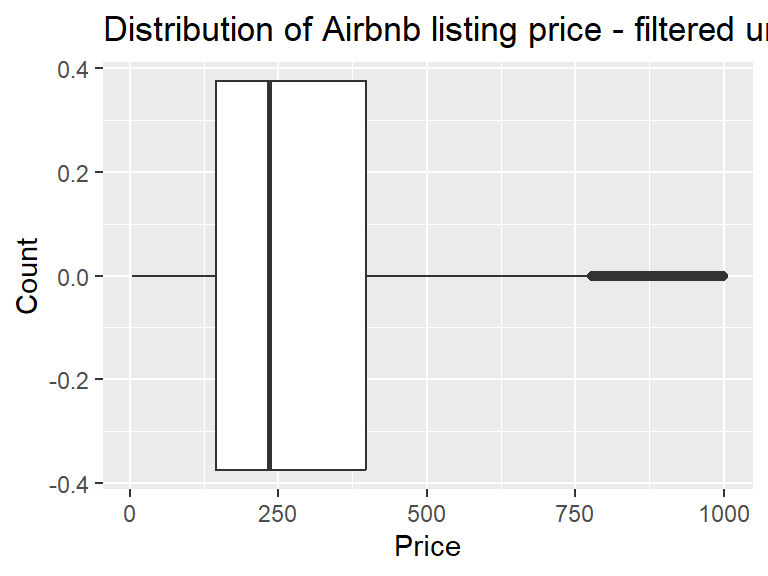
ablt1k |>
  summarise(
    min = min(price, na.rm = TRUE),
    mean = mean(price, na.rm = TRUE),
    median = median(price, na.rm = TRUE),
    sd = sd(price, na.rm = TRUE),
    iqr = IQR(price, na.rm = TRUE),
    max = max(price, na.rm = TRUE)
  )
# A tibble: 1 × 6
min mean median sd iqr max
<dbl> <dbl> <dbl> <dbl> <dbl> <dbl>
1 4.14 294. 234 207. 252. 1000.Keeping only listings priced at $1,000 or less removed 384 listings (about 6.5% of the 5,932 with a price). The distribution is still right skewed, but much less than before. The mean ($294) is now fairly close to the median ($234), where before it was nearly double. The max changed the most, which is expected since that is what we filtered on. Of the rest, the standard deviation changed the most, falling from $1,432 to $207 now that the extreme prices are gone. The min did not change at all ($4.14) and the median changed the least of the others, dropping from $252 to $234, because the median isn’t pulled around by extreme values. The IQR dropped a little, from $287 to $252.
6. Filtered price distribution by room type
Using only listings with prices at or below $1000, create a faceted histogram where each facet represents a room type (room_type) and displays the distribution of Airbnb prices (price) for that room type. Compare the frequency of responses and skew of prices across these different room types. Comment on one thing that you noticed.
ablt1k |>
  ggplot(aes(x = price)) +
  geom_histogram(binwidth = 50) +
  facet_wrap(~room_type) +
  labs(x = "Price", y = "Count",
       title = "Distribution of Airbnb listing price by room type")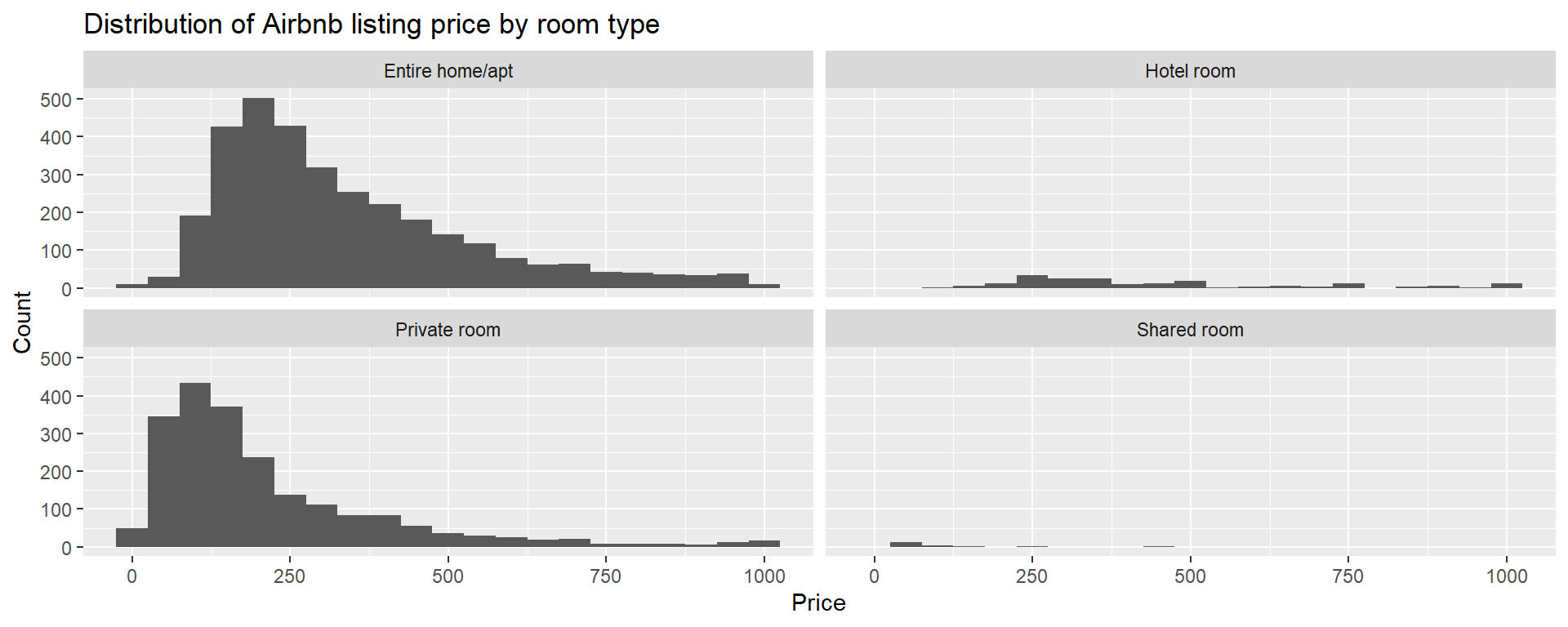
Among listings priced at $1,000 or less, both the number of listings and the shape of the price distribution differ by room type. Entire homes and private rooms make up nearly all of the listings, and there are very few hotel rooms and shared rooms. Entire homes and private rooms are both right skewed, with private rooms more strongly skewed: most private rooms are under $300, with a long thin tail off to the right. Hotel room prices are spread out between about $100 and $1,000, with roughly half falling between $200 and $400. There are very few hotel or shared rooms listed, most of them are priced at about $100 or less.
7. Filtered summary statistics by room type
Using only listings with prices at or below $1000, calculate the minimum, mean, median, standard deviation, IQR, and maximum listing price for each room type. Use the visualization and the summary statistics together to describe the distribution of listing prices by room type. Point out any oddities in the numbers.
ablt1k |>
  group_by(room_type) |>
  summarise(
    n = n(),
    min = min(price, na.rm = TRUE),
    mean = mean(price, na.rm = TRUE),
    median = median(price, na.rm = TRUE),
    sd = sd(price, na.rm = TRUE),
    iqr = IQR(price, na.rm = TRUE),
    max = max(price, na.rm = TRUE)
  )
# A tibble: 4 × 8
room_type n min mean median sd iqr max
<chr> <int> <dbl> <dbl> <dbl> <dbl> <dbl> <dbl>
1 Entire home/apt 3232 8.03 337. 278. 200. 246. 1000.
2 Hotel room 194 112. 447. 365 238. 277. 999
3 Private room 2102 4.14 215. 155 188. 194. 999
4 Shared room 20 46.5 97.3 64.5 94.7 32.2 451.Hotel rooms have the highest median price ($365), followed by entire homes ($278), private rooms ($155) and shared rooms ($64.50). Every room type has a mean above its median, confirming the right skew, and the gap is biggest for hotel rooms ($447 compared with $365). Hotel rooms are also the most spread out, with the largest SD ($238) and IQR ($277), while shared rooms are the least spread out (IQR = $32), though there are only 20 of them. A few numbers look off. An entire home listed for only $8.03 seems like a typo or error of some sort, and so do the $999 maximums for hotel and private rooms. Humans tend to round, so why $999?
8. Review scores across room types
Create a visualization that helps you compare the distribution of review scores (review_scores_rating) across room types. Include a brief interpretation of how Airbnb guests rate properties in general and how room types compare to each other.
ggplot(airbnb, aes(x = review_scores_rating,
                   y = reorder(room_type, review_scores_rating,
                               median, na.rm = TRUE))) +
  geom_boxplot(na.rm = TRUE) +
  labs(x = "Review score rating", y = "Room type",
       title = "Review scores by room type")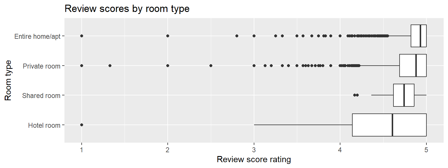
Review scores are high for every room type, with the boxes sitting near the top of the 1 to 5 scale, so most San Francisco Airbnb guests rate their stays highly. Entire homes have the highest median rating (about 4.9), followed by private rooms and shared rooms. Hotel rooms have the lowest median rating (about 4.6) and by far the widest box, so their ratings vary the most. The entire home, private room and hotel room boxplots all show low outliers, which means a small number of listings got much lower ratings than is typical. Overall the differences in ratings are small compared with the differences in price, but it is interesting that hotel rooms are the most expensive room type and also have the lowest median rating.
9. Is rating associated with price?
Create 2-3 scatterplots of price as the explanatory variable (on the x axis) against rating (as the response on the y axis). You could look at the pattern in the full data set, but likely to gain any meaningful information you will need to use a filtered data set (you can choose the dollar amount to filter on). You can color by a third variable if you choose to. Write 1-2 sentences about each plot sharing what you learned from that plot. Lastly try to answer the question “Do the highest reviewed places tend to be more expensive?”
ggplot(airbnb, aes(x=price, y = review_scores_rating)) +
  geom_point() + geom_smooth(se=FALSE)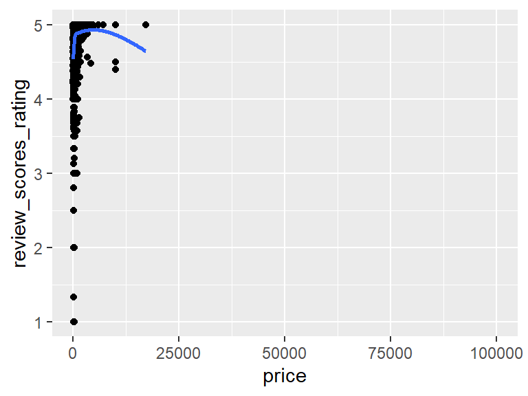
cor(airbnb$price, airbnb$review_scores_rating, use="pairwise.complete.obs")[1] 0.09159522Looking at the entire data set in one plot there isn’t much to see. The extreme prices squish almost all of the points up against the left side, and the correlation is 0.092, which is negligible.
ggplot(ablt1k, aes(x=price, y = review_scores_rating)) +
  geom_point() + geom_smooth(se=FALSE) + facet_wrap(~room_type)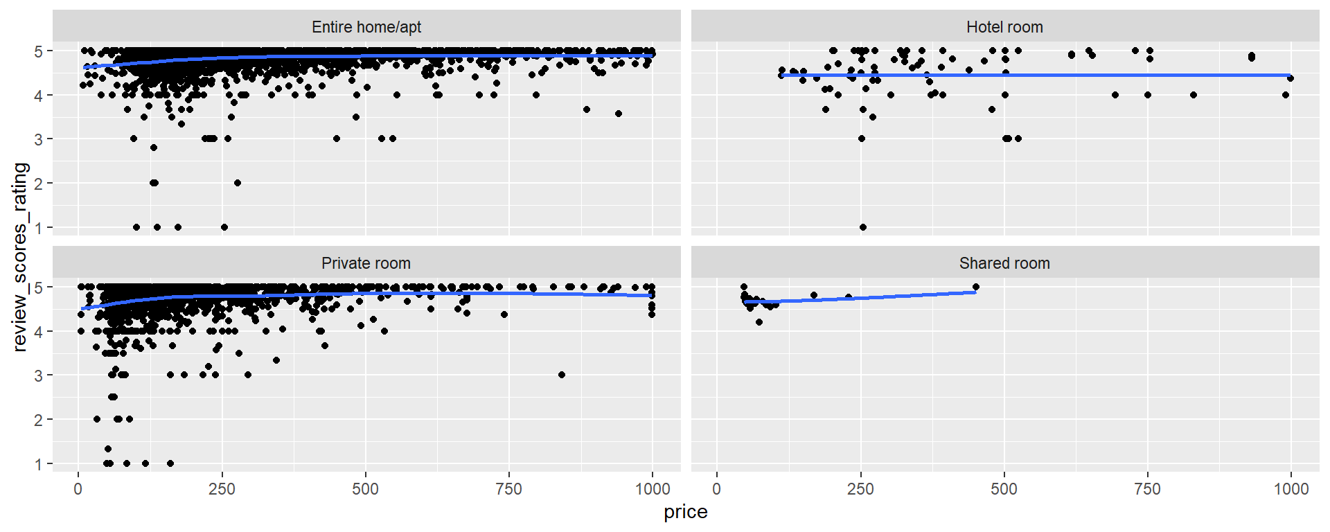
ablt1k |>
  group_by(room_type) |>
  summarize(cor = cor(price, review_scores_rating, use="pairwise.complete.obs"))
# A tibble: 4 × 2
room_type cor
<chr> <dbl>
1 Entire home/apt 0.139
2 Hotel room 0.0578
3 Private room 0.138
4 Shared room 0.412 For listings priced at $1,000 or less there is a small positive association between price and rating, but it is weak. The correlations for entire homes (0.139), private rooms (0.138) and hotel rooms (0.058) are all negligible. The smooth lines generally show ratings rising with price up to about $250 and then leveling off, which is likely because ratings cap out at 5 stars. Shared rooms have the highest correlation (0.412), but there are only 20 of them, so I wouldn’t read much into it. So do the highest reviewed places tend to be more expensive? A little. Ratings go up as price goes up through the lower prices, but past about $250 more money doesn’t buy much of a higher rating.
10. What makes a good listing?
Revisit the data documentation and explore the relationship between some other measures that we have not looked at yet, and either the price, or the rating of a listing. Create at least 2-3 graphs to explore your chosen relationship, calculate appropriate summary statistics and summarize what you’ve learned.
Note
This page adapts Data Science in a Box (HW 02: “Airbnb listings in Edinburgh”) by Mine Çetinkaya-Rundel, licensed under CC BY-SA 4.0. Source: tidyverse/datascience-box. Modifications include github language, changing datasets & specific questions.