library(tidyverse)
library(usdata)
library(sjPlot)
library(gtsummary)

gerrymander <- usdata::gerrymanderAE03 - Exploring gerrymandring (key)
Suggested answers
Important
These are suggested answers. This document is a reference, not an exhaustive key.
Note
Need a refresher on a plot type? Math 130’s plot reference guide is a good place to look.
Purpose
Gerrymandering is when a district’s boundaries are drawn to favor one political party (e.g. packing opposing voters into one district, or splitting them across several so they can’t win any). Lets explore some data on the 2016 election and outcomes related to the votes and gerrymandering.
- Translate English questions into code, using the data dictionary to find variable names
- Revisit and adapt code you’ve already written
- Back up every answer with specifics from your visualization — code alone isn’t an answer
Caution
Note that there are many ways to answer these questions. Some functions are suggested for you to use. You can choose your own adventure, but 1) you must use functions we have taught in this class so far, and 2) you should compare to your neighbor to make sure you are getting the same numbers.
Getting started
Load packages and get the gerrymander data out of the usdata package.
View the data using glimpse.
glimpse(gerrymander)Rows: 435
Columns: 12
$ district <chr> "AK-AL", "AL-01", "AL-02", "AL-03", "AL-04", "AL-05", "AL-0…
$ last_name <chr> "Young", "Byrne", "Roby", "Rogers", "Aderholt", "Brooks", "…
$ first_name <chr> "Don", "Bradley", "Martha", "Mike D.", "Rob", "Mo", "Gary",…
$ party16 <chr> "R", "R", "R", "R", "R", "R", "R", "D", "R", "R", "R", "R",…
$ clinton16 <dbl> 37.6, 34.1, 33.0, 32.3, 17.4, 31.3, 26.1, 69.8, 30.2, 41.7,…
$ trump16 <dbl> 52.8, 63.5, 64.9, 65.3, 80.4, 64.7, 70.8, 28.6, 65.0, 52.4,…
$ dem16 <dbl> 0, 0, 0, 0, 0, 0, 0, 1, 0, 0, 0, 0, 1, 0, 1, 0, 0, 0, 1, 0,…
$ state <chr> "AK", "AL", "AL", "AL", "AL", "AL", "AL", "AL", "AR", "AR",…
$ party18 <chr> "R", "R", "R", "R", "R", "R", "R", "D", "R", "R", "R", "R",…
$ dem18 <dbl> 0, 0, 0, 0, 0, 0, 0, 1, 0, 0, 0, 0, 1, 1, 1, 0, 0, 0, 1, 0,…
$ flip18 <dbl> 0, 0, 0, 0, 0, 0, 0, 0, 0, 0, 0, 0, 0, 1, 0, 0, 0, 0, 0, 0,…
$ gerry <fct> mid, high, high, high, high, high, high, high, mid, mid, mi…Each row is a US Congressional district. Here’s every variable in the data:
| variable | meaning |
|---|---|
district |
Congressional district ID |
state |
State the district is in |
party16 |
Party that won the district’s House election in 2016 |
clinton16 / trump16 |
Percent of the vote each candidate got in that district in the 2016 presidential election |
dem16 |
Whether a Democrat won that district’s House seat in 2016 |
party18 |
Party that won the district’s House election in 2018 |
dem18 |
Whether a Democrat won that district’s House seat in 2018 |
flip18 |
Whether the district’s House seat flipped from Republican to Democrat in the 2018 election. (0: no flip, -1: D to R, 1: R to D) |
gerry |
Prevalence of gerrymandering — low, mid, or high. “Prevalence” here just means how strongly that district’s lines were drawn that way — not whether it happened at all, but how much. |
This view, a table or document that connects a variable name (computer readable) to the meaning of the variable (human readable) is called a data dictionary or codebook.
Explore
1. Congressional districts per state
Which state has the most congressional districts? The least? How many congressional districts are there in this state? Use functions such as table, tbl_summary or count.
gerrymander |> count(state, sort = TRUE)# A tibble: 50 × 2
state n
<chr> <int>
1 CA 53
2 TX 36
3 FL 27
4 NY 27
5 IL 18
6 PA 18
7 OH 16
8 GA 14
9 MI 14
10 NC 13
# ℹ 40 more rowsgerrymander |> count(state) |> arrange(n)# A tibble: 50 × 2
state n
<chr> <int>
1 AK 1
2 DE 1
3 MT 1
4 ND 1
5 SD 1
6 VT 1
7 WY 1
8 HI 2
9 ID 2
10 ME 2
# ℹ 40 more rowsCalifornia has the most districts at 53, then Texas at 36. Several states: AK, DE, MT, ND, SD, VT and WY have only one.
2. Districts at the tails
Make side-by-side box plots of percent of vote received by Trump in the 2016 Presidential Election by prevalence of gerrymandering. Identify any Congressional Districts that are potential outliers — points that fall well outside the whiskers of their box, meaning that district’s Trump vote share was unusually high or low compared to other districts with the same gerrymandering prevalence. What information can you share about them?
ggplot(gerrymander, aes(x = trump16, y = gerry)) +
  geom_boxplot()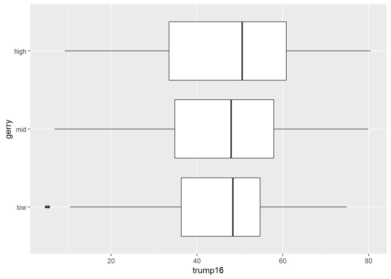
There are two districts where the share of Trump voters was unsually low amount of gerrymandering compared to other districts. Let’s find out who they are:
gerrymander |>
  filter(gerry == "low", trump16 < 10)
# A tibble: 2 × 12
district last_name first_name party16 clinton16 trump16 dem16 state party18
<chr> <chr> <chr> <chr> <dbl> <dbl> <dbl> <chr> <chr>
1 NY-13 Espaillat Adriano D 92.3 5.4 1 NY D
2 NY-15 Serrano Jose D 93.8 4.9 1 NY D
# ℹ 3 more variables: dem18 <dbl>, flip18 <dbl>, gerry <fct>Districts 13 and 15 in New York are the outliers. Both candidates are Democrat and received less than 6% of the vote for Trump, and the seat did not flip to republican.
3. Gerrymandering and flipping
This relationship can be looked at from two directions — does gerrymandering predict a 2018 flip, and does a 2018 flip predict gerrymandering? Support both with a visualization and summary statistics. The plot answers “what does the mix look like within each group?”; the table gives the exact proportions the plot is showing. Write 1-2 bullet points about what you noticed from each plot. Use specific numbers from the in your answer.
Direction 1: Is a Congressional District more likely to have high prevalence of gerrymandering if a Democrat was able to flip the seat in the 2018 election? To compare the breakdown of gerrymandering prevalence within each flipped group, make sure flip18 is on the x axis and that your percents add up to 100% within each category.
plot_xtab(x = gerrymander$flip18, grp = gerrymander$gerry, show.total = FALSE, margin = "row")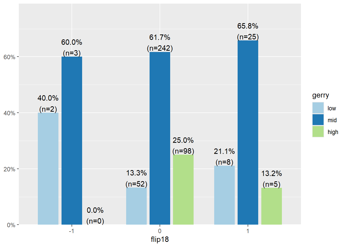
- One quarter of districts that did not flip have a high prevelance of gerrymandering.
- All counties that flipped Democrat to Republican have either low (40%) or mid (60%) prevelance of gerrymandering.
Direction 2: Is a Congressional District more likely to be flipped to a Democratic seat if it has high prevalence of gerrymandering, or low prevalence? Same two variables, just flipped — so now gerry is on the x-axis. Again, make sure your percents add up to 100% within each category.
plot_xtab(x = gerrymander$gerry, grp = gerrymander$flip18, show.total = FALSE, margin = "row")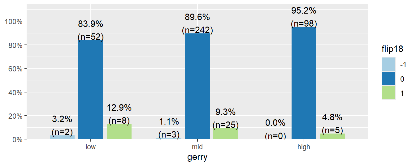
- The vast majority of seats didn’t flip (83.9% to 95.2%)
- 13% of districts with low prevalence of gerrymandering flipped to republican, compared to 5% in districts with high prevelance of gerrymandring.
4. Gerrymandering and presidential margin
Using mutate, create a new variable, margin16, measuring how many percentage points Clinton won or lost by in each district (clinton16 - trump16). Does gerrymandering prevalence relate to how lopsided the 2016 presidential race was in that district? Report the min, mean, and max margin by gerry level, then visualize the full distribution with a violin + boxplot combo.
gerrymander |>
  mutate(margin16 = clinton16 - trump16) |>
  group_by(gerry) |>
  summarise(
    min_margin = min(margin16),
    mean_margin = mean(margin16),
    max_margin = max(margin16)
  )
# A tibble: 3 × 4
gerry min_margin mean_margin max_margin
<fct> <dbl> <dbl> <dbl>
1 low -54.9 6.32 88.9
2 mid -63 3.25 82.8
3 high -63 1.34 78.2gerrymander |>
mutate(margin16 = clinton16 - trump16) |>
ggplot(aes(x = gerry, y = margin16, fill = gerry)) +
geom_violin(alpha = 0.5) +
geom_boxplot(width = 0.15, alpha = 0.5, show.legend = FALSE) +
stat_summary(fun = mean, geom = "point", shape = 18, size = 3, color = "black") +
labs(
x = "Gerrymandering prevalence",
y = "2016 margin (Clinton % − Trump %)",
fill = "Gerrymandering prevalence"
) + coord_flip()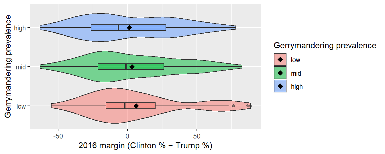
- Low prevalence: Roughly symmetric near the middle, but pulled right by two big outliers (the New York districts we found in “Districts at the tails”) — mean margin is +6.3, well above the median, which sits close to 0. Middle 50% of districts range roughly -15 to +20; full spread runs -54.9 to 88.9.
- Mid prevalence: Fairly symmetric and unimodal, no real outliers beyond the whiskers. Center is close to even (mean +3.3), spread is a bit wider than low (-63 to 82.8).
- High prevalence: Slightly bimodal — one bulge below 0, a second smaller bulge up around +50 — and the median actually sits below 0, even though the mean (+1.3) is still barely positive because of a handful of lopsided pro-Clinton districts pulling it up. Spread is about the same width as mid (-63 to 78.2).
Overall: as gerrymandering prevalence goes up, the mean margin shrinks toward 0 (6.3 –> 3.3 –> 1.3) and the median district tips slightly toward Trump. More heavily gerrymandered districts look competitive-to-Republican-leaning on the whole, even though a few landslide Democratic districts keep pulling the average up.
NoteAcknowledgements and references
This page adapts material from STA199 (Duke, Fall 2025) by Mine Çetinkaya-Rundel, AEs 03 (“Gerrymandering + data exploration I”) and 04 (“Gerrymandering + data exploration II”)