Hello, World!

Lecture 1

Author
Affiliation

Dr. Robin Donatello

Chico State
DATA 385 - Fall 2026

Published

August 25, 2026

Hello world!

Meet the prof

Dr. Robin Donatello

  • Professor of Statistics (and Data Science)
  • Proud alum from Butte College & Chico State (BS Biology, BS Statistics, minor in Chemistry)
  • Doctorate in Public Health - Biostatisics from UCLA
  • Director of the Wildcat Data Hub and the Data Science Initiative at Chico State
  • Data Manager at the Center for Healthy Communities
  • Pitbull mamma, veggie gardner, and gamer (TTRPG and video games)

Office: Holt 202 Office hours:

  • Mon 1-2pm, T/R 2-3pm in Holt 202
  • Wed 1-3pm at Community Coding
  • By appointment (booking link in Canvas, on syllbus and on my website)

Meet each other!

Please share with at least two classmates…

  • Your name
  • Your year
  • Where you’re from
  • What you did this past summer
  • What you hope to get out of this course

Meet data science

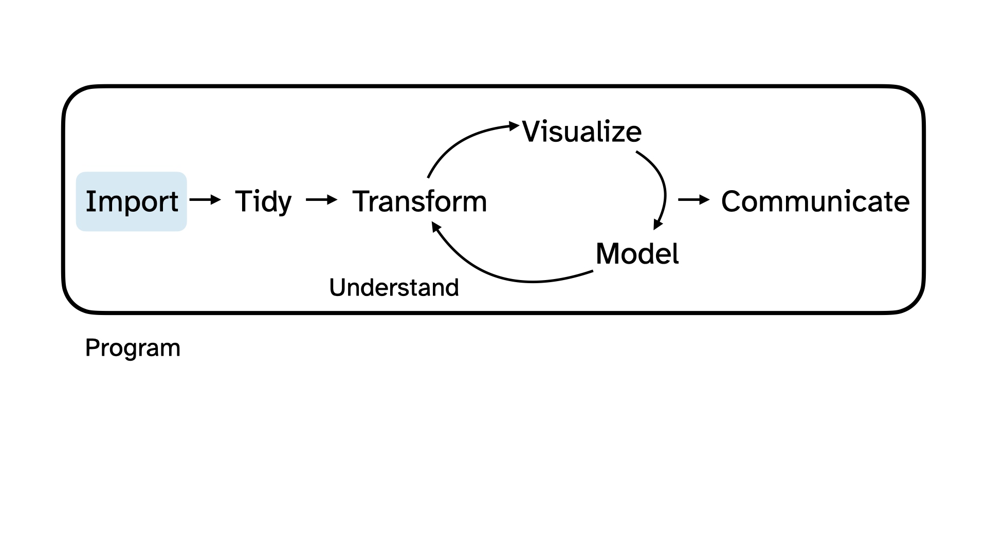
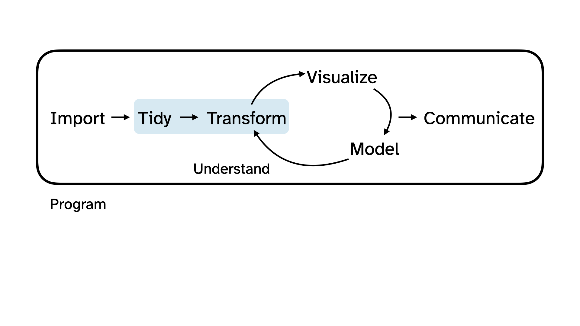
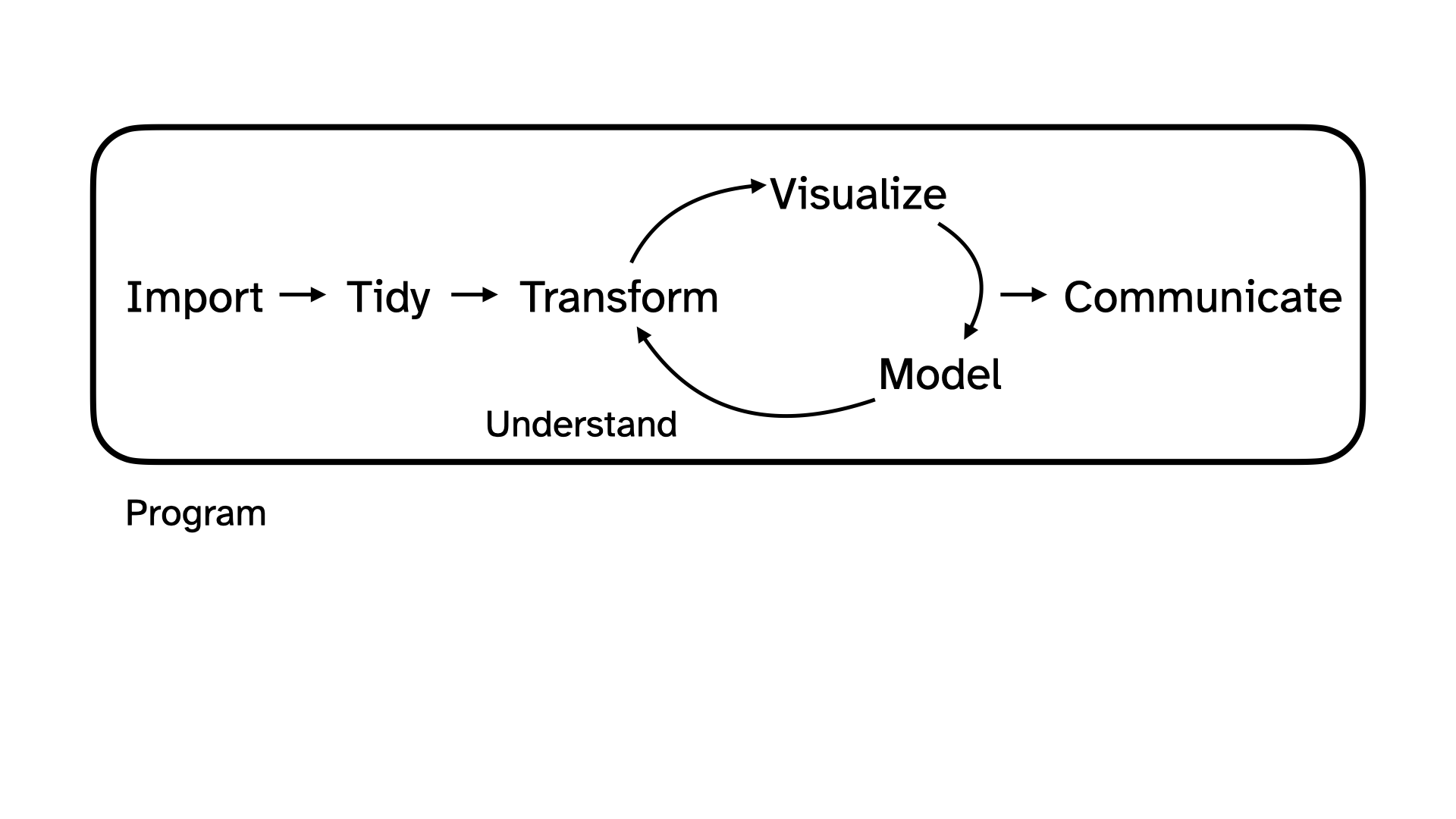
Data science cycle: Import, tidy, transform, visualize, model, communicate.

  • Data science is an exciting discipline that allows you to turn raw data into understanding, insight, and knowledge.

  • We’re going to learn to do this in a modern and tidy way – more on that later!

  • This is a course on introduction to data science, with an emphasis on statistical thinking.

Let’s do some data science!

Data Collection

  • Yesterday we collected some data from you!
  • Today we’re going to explore that data together, following the data science cycle.
  • Didn’t take it yet? Scan the QR code and do it now!

QR code linking to the survey.

Beginning the data science cycle

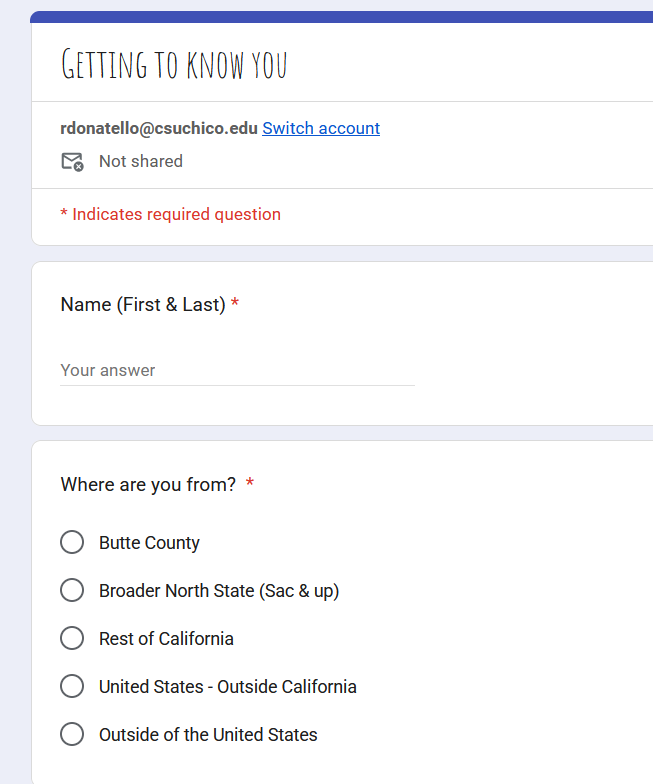
You took a survey, built in Google Forms:

Screenshot of Getting to know you survey on Google.

We want to explore that data and get to know you!

Load some packages

More on what packages are on Thursday, but in a nutshell “get your tools out of the toolbox”:

Code
library(tidyverse)   # for data wrangling and visualization
library(scales)      # for better axis labels
library(tidytext)    # for handling text data
library(ggwordcloud) # for the learn-best word cloud
library(zipcodeR)    # for the hometown map
library(maps)        # also for mapping
library(ggpubr)      # for better density plot

Import

Data science cycle: Import, tidy, transform, visualize, model, communicate. Import is highlighted.

Import the data

We could download the data and save it as a csv file on our computer, edit out the student names, name it survey-anonymized.csv and save it in a folder called data. Then we would import it into R using the read_csv() function:

Code
survey <- read_csv(here::here("slides/data", "survey-anonymized.csv"))
Rows: 20 Columns: 7
── Column specification ──────────────────────────────────────────────
Delimiter: ","
chr (6): zipcode, stats_experience, programming_experience, progra...
dbl (1): commute_minutes

ℹ Use `spec()` to retrieve the full column specification for this data.
ℹ Specify the column types or set `show_col_types = FALSE` to quiet this message.

Import the data - Live connection

Alternatively, we can authorize R to directly read the Google Sheet that holds the responses from the Google Form you filled out.

Code
survey <- read_sheet("https://docs.google.com/spreadsheets/d/1R4_afqSB6KXD9HwfYP-wjMqvwxiDTGEMATmWmkqqXig")

Take a peek 👀 at the data

Code
survey
# A tibble: 20 × 7
   zipcode stats_experience                     programming_experience
   <chr>   <chr>                                <chr>                 
 1 95928   Yes, I have taken a high school sta… A little — I've writt…
 2 95818   No, I have not taken any statistics… None                  
 3 95926   Yes, I have taken another college c… Some — I've worked on…
 4 90210   No, I have not taken any statistics… A lot — I use program…
 5 95965   Yes, I have taken a high school sta… None                  
 6 96001   No, I have not taken any statistics… A little — I've writt…
 7 97201   Yes, I have taken another college c… Some — I've worked on…
 8 95973   No, I have not taken any statistics… A lot — I use program…
 9 93701   Yes, I have taken a high school sta… A little — I've writt…
10 95991   No, I have not taken any statistics… None                  
11 95926   Yes, I have taken another college c… Some — I've worked on…
12 00000   No, I have not taken any statistics… A little — I've writt…
13 95928   Yes, I have taken a high school sta… None                  
14 90210   No, I have not taken any statistics… A lot — I use program…
15 95814   Yes, I have taken another college c… Some — I've worked on…
16 95965   No, I have not taken any statistics… A little — I've writt…
17 85001   Yes, I have taken a high school sta… None                  
18 92101   No, I have not taken any statistics… Some — I've worked on…
19 95973   Yes, I have taken another college c… A lot — I use program…
20 96001   No, I have not taken any statistics… A little — I've writt…
# ℹ 4 more variables: programming_languages <chr>,
#   data_interests <chr>, learn_best <chr>, commute_minutes <dbl>

Statistics experience

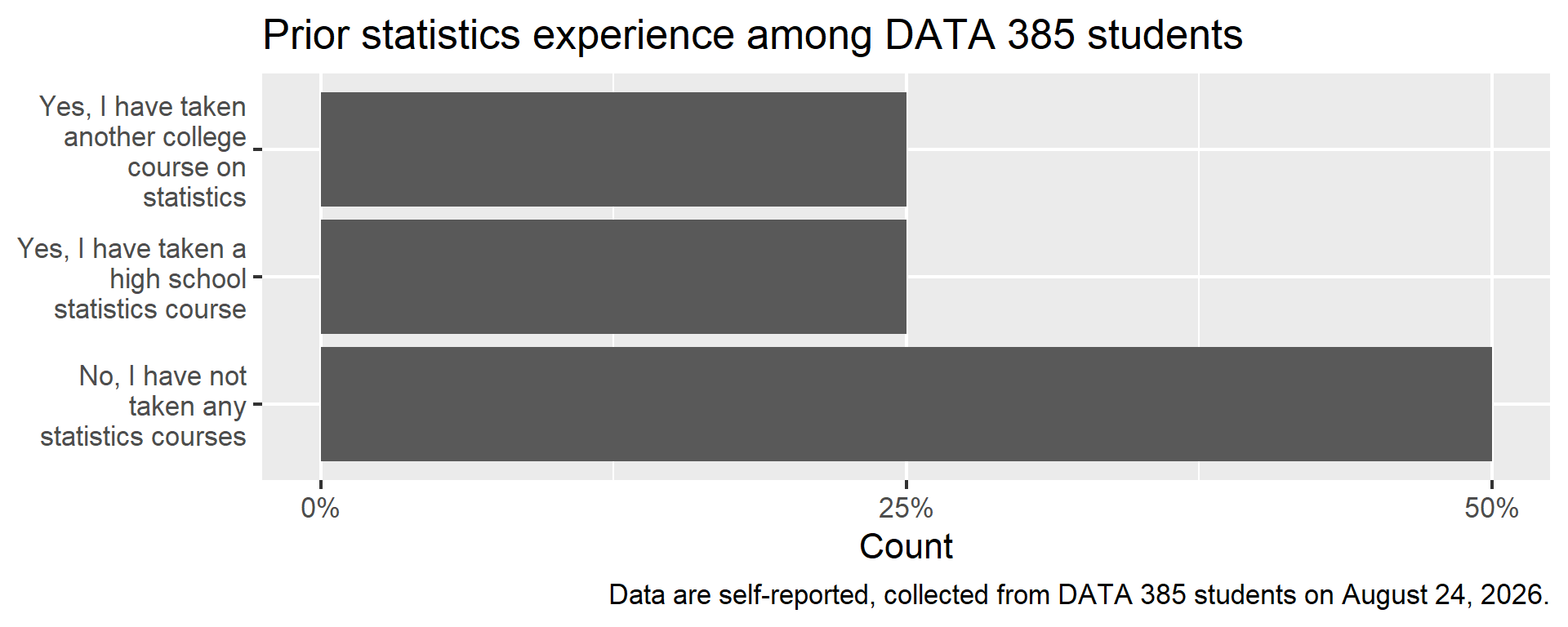
We asked you the following multiple-choice question where you could only pick one option:

Have you taken any statistics courses before?

  • Yes, I have taken another college course on statistics
  • Yes, I have taken a high school statistics course
  • No, I have not taken any statistics courses

Visualize

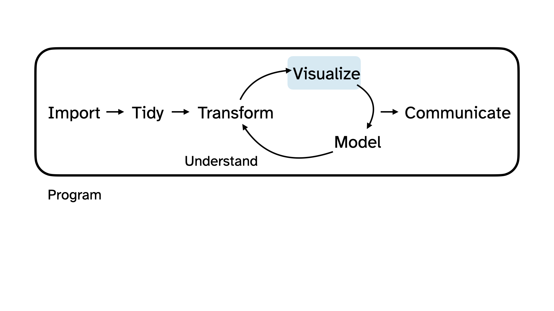
One way to make sense of data collected via a question like this is to visualize it.

Data science cycle: Import, tidy, transform, visualize, model, communicate. Visualize is highlighted.

Visualize

Code
survey |>
  count(stats_experience) |>
  mutate(prop = n / sum(n)) |>
  ggplot(aes(y = stats_experience, x = prop))+
  geom_col(show.legend = FALSE) +
  scale_y_discrete(labels = label_wrap(20)) +
  scale_x_continuous(labels = percent_format(accuracy = 1), breaks = c(0, 0.25, 0.5)) +
  labs(
    title = "Prior statistics experience among DATA 385 students",
    y = NULL,
    x = "Count"
  ) +
  labs(
    caption = "Data are self-reported, collected from DATA 385 students on August 24, 2026."
  )

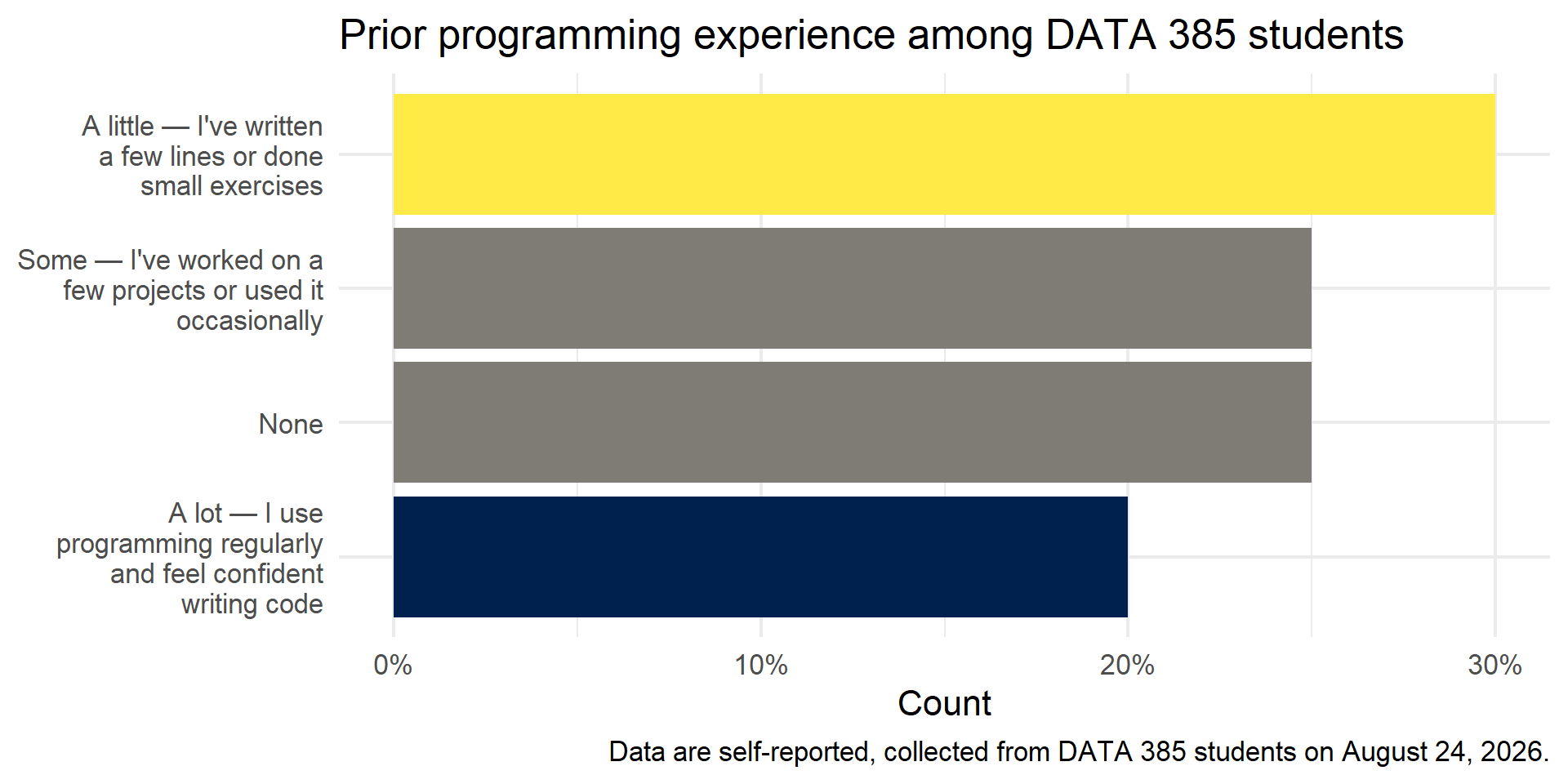
Programming experience

We also asked you the following multiple-choice question where you could only pick one option:

How much experience do you have with programming?

  • None
  • A little — I’ve written a few lines or done small exercises
  • Some — I’ve worked on a few projects or used it occasionally
  • A lot — I use programming regularly and feel confident writing code

Visualize

Code
survey |>
  count(programming_experience) |>
  mutate(prop = n / sum(n)) |>
  ggplot(aes(y = fct_reorder(programming_experience, prop), x = prop, fill = prop))+
  geom_col(show.legend = FALSE) +
  scale_y_discrete(labels = label_wrap(25)) +
  scale_x_continuous(labels = percent_format(accuracy = 1), breaks = c(0, 0.1, 0.2, 0.3, 0.4)) +
  scale_fill_viridis_c(option = "E") +
  labs(
    title = "Prior programming experience among DATA 385 students",
    y = NULL,
    x = "Count"
  ) +
  labs(
    caption = "Data are self-reported, collected from DATA 385 students on August 24, 2026."
  ) +
  theme_minimal(base_size = 16)

Learn best

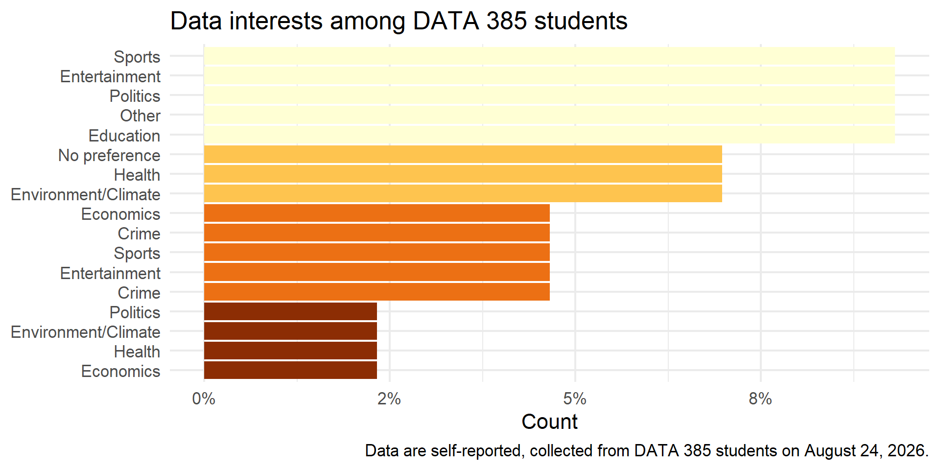
We also asked you the following multiple-choice question where you could as many options as you liked:

What types of data interest you?

  • Crime
  • Economics
  • Education
  • Entertainment (e.g., books, movies, music)
  • Environment/Climate
  • Health (e.g., social determinants of health, medical)
  • Politics
  • Sports
  • Other
  • No preference

Peek at the data 👀

Code
survey |>
  select(data_interests)
# A tibble: 20 × 1
   data_interests                                                     
   <chr>                                                              
 1 Sports, Entertainment (e.g., books, movies, music)                 
 2 Crime, Politics                                                    
 3 Health (e.g., social determinants of health, medical), Environment…
 4 Economics, Sports, Politics                                        
 5 Entertainment (e.g., books, movies, music), Education              
 6 No preference                                                      
 7 Environment/Climate                                                
 8 Sports, Entertainment (e.g., books, movies, music), Other          
 9 Health (e.g., social determinants of health, medical), Education, …
10 Politics, Economics                                                
11 No preference                                                      
12 Sports, Environment/Climate                                        
13 Entertainment (e.g., books, movies, music), Other                  
14 Economics, Crime, Politics                                         
15 Health (e.g., social determinants of health, medical), Education   
16 Sports, Politics, Other                                            
17 Entertainment (e.g., books, movies, music), Environment/Climate, E…
18 No preference                                                      
19 Crime, Health (e.g., social determinants of health, medical), Spor…
20 Entertainment (e.g., books, movies, music), Other                  
Tidy + Transform

Before we can visualize this variable, we need to tidy and transform it.

Data science cycle: Import, tidy, transform, visualize, model, communicate. Tidy and transform are highlighted.

Tidy + Transform

Code
survey |>
  # remove text in parentheses
  mutate(data_interests = str_remove_all(data_interests, "\\s*\\(.*?\\)")) |>
  # separate into multiple rows for each interest, using comma as delimiter
  separate_longer_delim(data_interests, delim = ",") |>
  count(data_interests, sort = TRUE) |>
  mutate(prop = n / sum(n))
# A tibble: 17 × 3
   data_interests             n   prop
   <chr>                  <int>  <dbl>
 1 " Education"               4 0.0930
 2 " Other"                   4 0.0930
 3 " Politics"                4 0.0930
 4 "Entertainment"            4 0.0930
 5 "Sports"                   4 0.0930
 6 " Environment/Climate"     3 0.0698
 7 "Health"                   3 0.0698
 8 "No preference"            3 0.0698
 9 " Crime"                   2 0.0465
10 " Entertainment"           2 0.0465
11 " Sports"                  2 0.0465
12 "Crime"                    2 0.0465
13 "Economics"                2 0.0465
14 " Economics"               1 0.0233
15 " Health"                  1 0.0233
16 "Environment/Climate"      1 0.0233
17 "Politics"                 1 0.0233

Visualize

Code
survey |>
  mutate(data_interests = str_remove_all(data_interests, "\\s*\\(.*?\\)")) |>
  separate_longer_delim(data_interests, delim = ",") |>
  count(data_interests, sort = TRUE) |>
  mutate(prop = n / sum(n)) |>
  filter(!is.na(data_interests)) |>
  ggplot(aes(y = fct_reorder(data_interests, prop), x = prop, fill = prop)) +
  geom_col(show.legend = FALSE) +
  scale_y_discrete(labels = label_wrap(20)) +
  scale_x_continuous(labels = percent_format(accuracy = 1)) +
  scale_fill_distiller(palette = "YlOrBr") +
  labs(
    title = "Data interests among DATA 385 students",
    y = NULL,
    x = "Count",
    caption = "Data are self-reported, collected from DATA 385 students on August 24, 2026."
  ) +
  theme_minimal(base_size = 16)

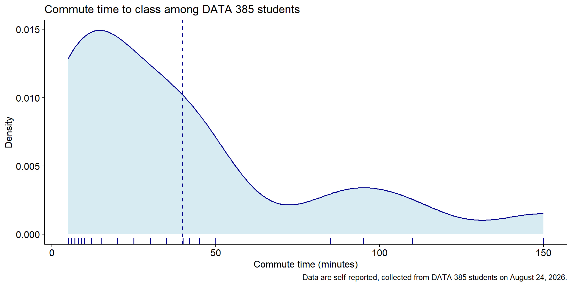
Commute time

We also asked you the following open-ended, numeric question:

How long does it take you to commute from home to this classroom in minutes?

Code
survey |>
  ggdensity(
    x = "commute_minutes",
    fill = "lightblue",
    color = "darkblue",
    add_density = TRUE,
    add = "mean",
    rug = TRUE,
    title = "Commute time to class among DATA 385 students",
    xlab = "Commute time (minutes)",
    ylab = "Density"
  ) +
  labs(caption = "Data are self-reported, collected from DATA 385 students on August 24, 2026.")

Learn best

We also asked you the following open-ended question:

How do you learn best?

Code
survey |>
  select(learn_best)
# A tibble: 20 × 1
   learn_best                                                         
   <chr>                                                              
 1 I learn best by doing hands-on practice rather than just reading o…
 2 Visual explanations with diagrams help me a lot.                   
 3 I retain things best when I can teach them back to someone else.   
 4 I like working through lots of small examples until it clicks.     
 5 Repetition and flashcards work well for me.                        
 6 I need to see a real example before the concept makes sense.       
 7 I learn best in study groups where we talk through problems out lo…
 8 Building small projects on my own is how it really sinks in for me.
 9 I do best with step-by-step written instructions I can follow alon…
10 Lecture plus notes works fine for me  but I need to rewrite my not…
11 I'm a visual learner - charts and diagrams over text every time.   
12 I learn best by breaking things and figuring out how to fix them.  
13 Podcasts and videos stick with me better than reading textbooks.   
14 I like diving straight into the code and learning by debugging err…
15 Office hours and asking questions one-on-one really help me.       
16 I learn best from worked examples I can compare my own work agains…
17 I need to write things out by hand to actually learn them.         
18 Group projects where I can bounce ideas off others work best for m…
19 I'm most productive with a clear checklist and deadlines to work t…
20 Trial and error - I just start messing with things until they work.

Tidy + Transform + Summarize

We can use text mining techniques, like tokenizing to words to explore this open-ended question:

Code
survey |>
  select(learn_best) |>
  unnest_tokens(word, learn_best) |>
  anti_join(stop_words, by = "word") |>
  count(word, sort = TRUE) |>
  filter(n > 1) |>
  print(n = Inf)
# A tibble: 8 × 2
  word         n
  <chr>    <int>
1 learn        5
2 diagrams     2
3 examples     2
4 notes        2
5 projects     2
6 reading      2
7 step         2
8 visual       2

Tidy + Transform + Summarize

We can also tokenize to bigrams (pairs of words):

Code
survey |>
  select(learn_best) |>
  tidytext::unnest_tokens(bigrams, learn_best, token = "ngrams", n = 2) |>
  count(bigrams, sort = TRUE) |>
  filter(n > 1) |>
  print(n = Inf)
# A tibble: 10 × 2
   bigrams        n
   <chr>      <int>
 1 for me         4
 2 i can          4
 3 i learn        4
 4 learn best     4
 5 i need         3
 6 need to        3
 7 best by        2
 8 help me        2
 9 i like         2
10 my own         2

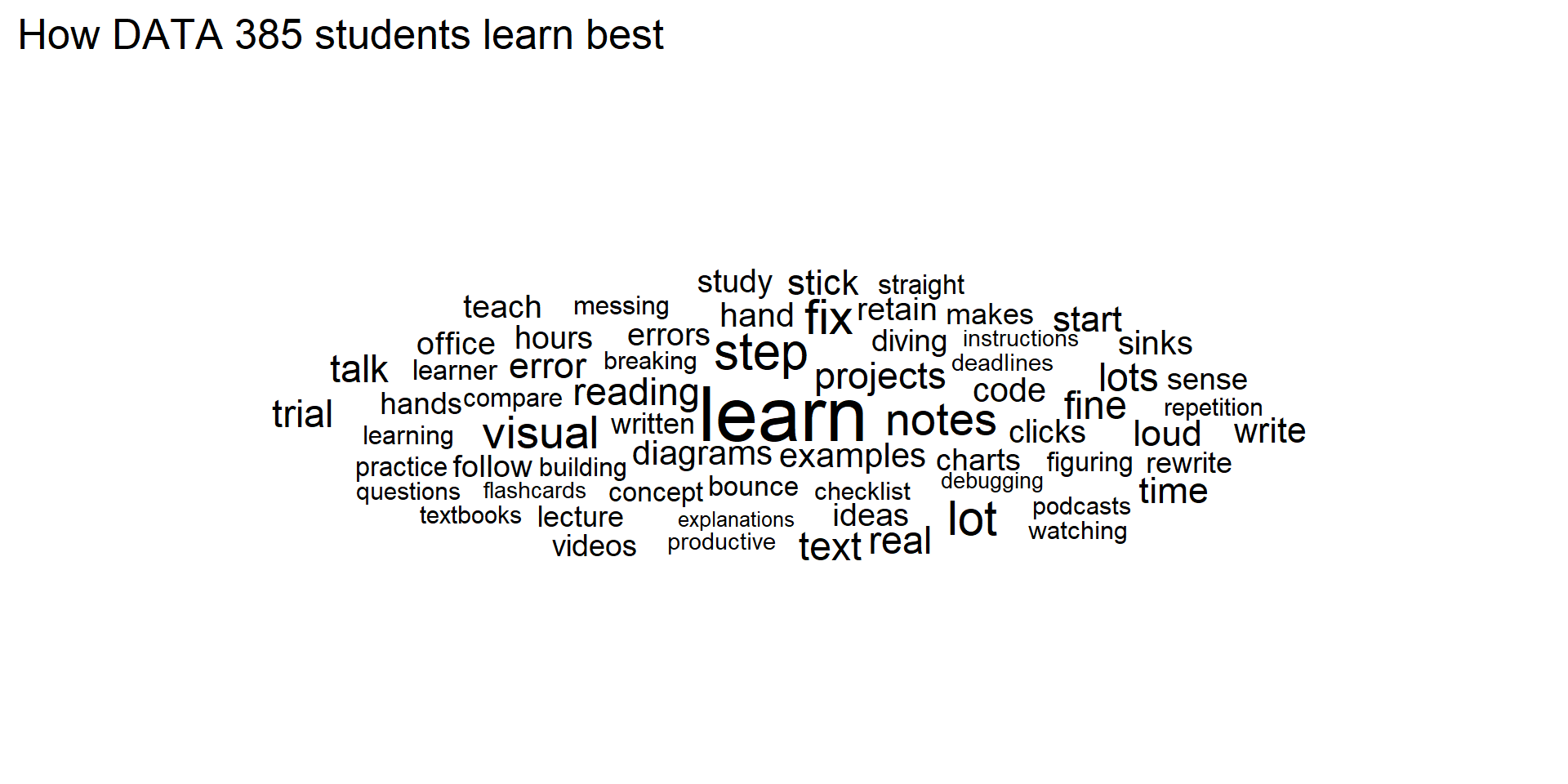
Tidy + Transform + Visualize: Word cloud

Code
survey |>
  select(learn_best) |>
  unnest_tokens(word, learn_best) |>
  anti_join(stop_words, by = "word") |>
  count(word, sort = TRUE) |>
  ggplot(aes(label = word, size = n)) +
  ggwordcloud::geom_text_wordcloud(area_corr = TRUE) +
  scale_size_area(max_size = 24) +
  labs(title = "How DATA 385 students learn best") +
  theme_minimal(base_size = 16)

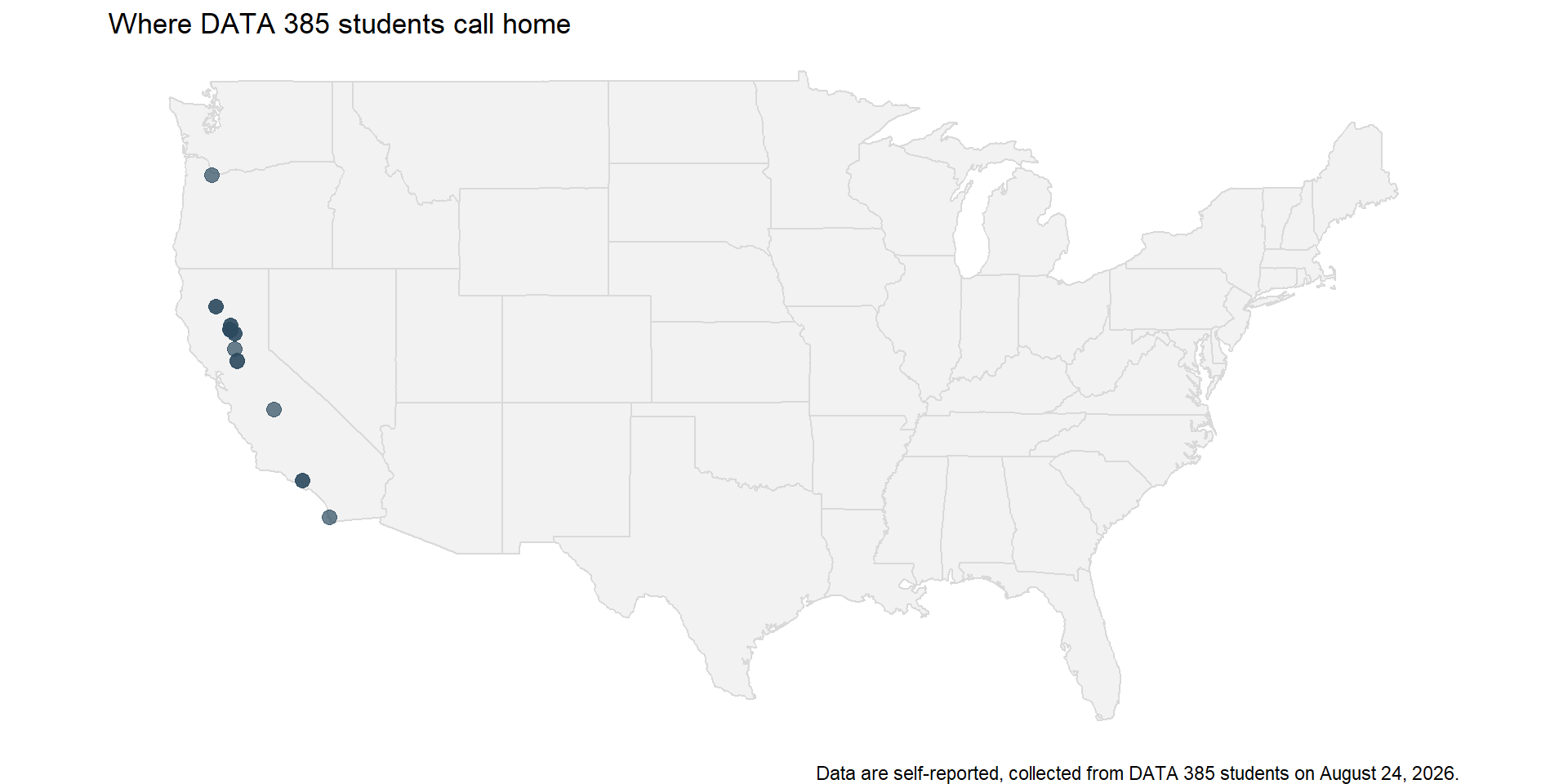
Where are you from?

We also asked you the following question:

What is the zipcode of your hometown?

If you are from out of country, please enter 00000.

Tidy + Transform + Visualize: Map

Code
survey_locations <- survey |>
  mutate(zipcode = str_pad(zipcode, width = 5, side = "left", pad = "0")) |>
  left_join(zip_code_db, by = "zipcode")

survey_locations |>
  filter(!is.na(lat), zipcode != "00000") |>
  ggplot(aes(x = lng, y = lat)) +
  borders("state", colour = "gray85", fill = "gray95") +
  geom_point(color = "#2C4A5E", size = 3, alpha = 0.7) +
  coord_quickmap() +
  theme_void() +
  labs(
    title = "Where DATA 385 students call home",
    caption = "Data are self-reported, collected from DATA 385 students on August 24, 2026."
  )
Warning: `borders()` was deprecated in ggplot2 4.0.0.
ℹ Please use `annotation_borders()` instead.

Note: rows with zipcode 00000 (international students) are excluded from the map — worth calling out as a group separately rather than silently dropping them.

Programming language comfort

We also asked you the following open-ended question:

If you’ve programmed before, which languages have you used, and how comfortable do you feel with each? If you haven’t programmed before, please leave this question blank.

Take a peek 💻

And the answers are non-trivial to tidy up, e.g.,

Code
survey |>
  select(programming_languages)
# A tibble: 20 × 1
   programming_languages                                              
   <chr>                                                              
 1 Python - just a intro course                                       
 2 <NA>                                                               
 3 Python - pretty comfortable, SQL - a little                        
 4 Java - very comfortable, Python - very comfortable, C++ - comforta…
 5 <NA>                                                               
 6 HTML/CSS - beginner                                                
 7 Python - comfortable, R - a little                                 
 8 Python - very comfortable, JavaScript - comfortable, Java - a litt…
 9 Python - a little from a summer camp                               
10 <NA>                                                               
11 Python - comfortable, MATLAB - a little                            
12 C - a little in high school                                        
13 <NA>                                                               
14 Python - very comfortable, C++ - very comfortable, Rust - a little 
15 R - comfortable, Python - a little                                 
16 Python - one intro class                                           
17 <NA>                                                               
18 JavaScript - comfortable, Python - a little                        
19 Python - very comfortable, SQL - comfortable, Java - comfortable   
20 Scratch - from a middle school class                               

Can AI help?

Prompt:

Summarize the following responses to the question “If you’ve programmed before, which languages have you used, and how comfortable do you feel with each? If you haven’t programmed before, please leave this question blank.”. Write your response in a short paragraph.

Response:

Python is by far the most common language, ranging from a little exposure (summer camp, one intro course) to very comfortable. Several students also have experience with a second language — Java, C++, and JavaScript each show up a few times, generally at moderate-to-strong comfort levels — while others mention lighter exposure to SQL, R, C, MATLAB, Rust, or HTML/CSS. A couple of students noted only minimal or early exposure (e.g., Scratch from middle school, C in high school). Overall, the class has a wide range of backgrounds, from complete beginners with just one intro course to students who are very comfortable across multiple languages.

Can it be trusted 100%?

No. They can be misleading, inaccurate, hallucinate or in general sound more confident than they are. Humans should always stay “in the loop”. Hence – the interdisciplinary approach!

Course overview

Homepage

https://data385.netlify.app/

  • All course materials
  • Links to Canvas, GitHub, JupyterHub, etc.

Key dates and logistics

  • Meeting time: TTh 12:30–1:45pm
  • Meeting location: TBD
  • Prerequisites: CSCI 111, MATH 130, or MATH 230; and MATH 109 or MATH 120
  • Add/Drop deadline: TBD

Course toolkit

  • R + RStudio via Posit Cloud in Week 1 — no installation needed on day one
  • Local installation of R + RStudio expected by Week 4
  • Git + GitHub required starting Week 1
  • Communication: Discord
  • Assignment submission and feedback: TBD
  • GitHub organization: github.com/DATA385-f26
  • RStudio containers: chicostate.jupyter.cal-icor.org
  • Textbooks - R4DS and IMS

A note on course videos

Most videos linked throughout this course come from Duke’s DS in a Box / STA 199 courses, recorded around 2020. A few things to watch for:

  • Some content is Duke-specific (their policies, their toolkit setup) — that’s expected, focus on the R/data science content itself
  • Terminology has shifted since 2020:
    • “R Markdown” → we use Quarto, its modern successor. Same core idea (code + narrative in one document), slightly different syntax
    • “RStudio Cloud” / “Posit Cloud” → we use RStudio via JupyterHub (Chico State’s setup)
  • If a video shows something unfamiliar, it’s probably just an older/different setup — not a mistake on your end. Ask if you’re not sure.

Weekly class flow

This is a flipped classroom: content prep happens before class, and class time is for code-alongs and collaborative work.

  • Sun: week’s assignments due by midnight
  • Mon: prepare for Tuesday’s class
  • Tue: class
  • Wed: prepare for Thursday’s class
  • Thu: class
  • Fri–Sun: complete that week’s homework/reading response, due Sunday at midnight
  • Activities started in class are due by the end of that class

AI policy

  • Phase 1 (~Weeks 1–8): no LLM use
  • Phase 2 (~Weeks 9–16): LLMs taught and used explicitly
  • More details throughout the semester

Attendance and participation

  • Participation: 5% of course grade
  • Format details: TBD

Active learning

  • Worksheets: TBD
  • Active learning format: TBD

Labs

  • 25% of course grade
  • Hands-on practice with data analysis
  • Additional format details: TBD

Homework & reading responses

  • 20% of course grade (combined)
  • Due Sunday at midnight each week (see Weekly class flow)
  • Late work: assignments close one week after the original due date, or 48 hours before an exam — whichever comes first
  • Reading response format: TBD

Quizzes & exams

  • Quizzes: 10% of course grade
  • Exams: 30% of course grade
  • Format details: TBD

Project

  • 10% of course grade
  • Final project details: TBD

Teams

  • TBD — not yet established whether labs or the project will be team-based

Grading

Category Percentage
Labs 25%
Homework/Reading Responses 20%
Exams 30%
Quizzes 10%
Project 10%
Participation 5%

Standard +/– letter scale: A (90–100), B (80–89), C (70–79), D (60–69), F (below 60)

See course syllabus for full grading policy details.

Wrap up - Next up

This week’s tasks