We put together what we’ve learned so far about importing data, data types and classes, and recoding data. We use them to make a visualization, and improve it one step at a time.
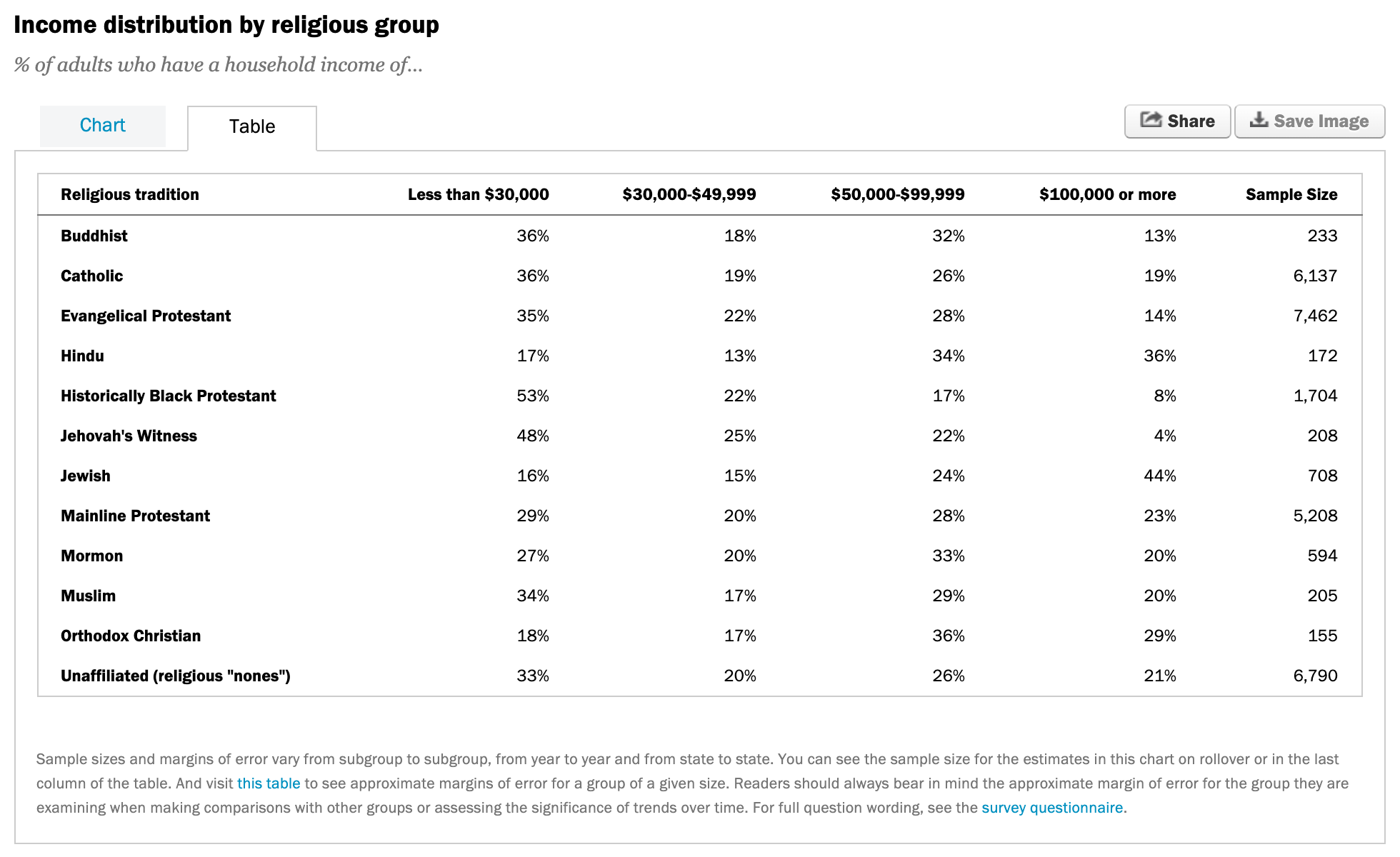
The Pew Research Center surveys people in the US on their religious tradition and their income. Each row is a religious tradition, each column is an income level, and the cells hold percentages. Pew has a button to download this data set, and that’s what we start with.
The data was saved as an Excel file, so we read it in with read_excel(). We get 12 rows and 6 columns, which matches the screenshot from the website. We call this data frame rel_inc.
The first column, Religious tradition, has a space in it. We also want to shorten Sample Size to n so it’s easier to refer to. The syntax for rename() is new_name = old_name. The old names have spaces, so they need backticks. Why not rename the other wonky names like $100,000 or more? We’re going to use those as values, not variable names, by pivoting.
Which function?
If we want a new variable called income with levels such as “Less than $30,000”, “$30,000-$49,999”, … etc. which function should we use?
# A tibble: 48 × 4
  religion     n income            proportion
  <chr>    <dbl> <chr>                  <dbl>
1 Buddhist   233 Less than $30,000       0.36
2 Buddhist   233 $30,000-$49,999         0.18
3 Buddhist   233 $50,000-$99,999         0.32
4 Buddhist   233 $100,000 or more        0.13
5 Catholic  6137 Less than $30,000       0.36
6 Catholic  6137 $30,000-$49,999         0.19
# ℹ 42 more rows
We start with 12 rows and 6 columns. We want 48 rows and 4 columns, where the income levels are stacked on top of each other instead of spread across the columns.
Pivot longer
rel_inc %>%rename(religion =`Religious tradition`, n =`Sample Size`) %>%pivot_longer(cols =-c(religion, n), # all but religion and nnames_to ="income",values_to ="proportion")
# A tibble: 48 × 4
  religion     n income            proportion
  <chr>    <dbl> <chr>                  <dbl>
1 Buddhist   233 Less than $30,000       0.36
2 Buddhist   233 $30,000-$49,999         0.18
3 Buddhist   233 $50,000-$99,999         0.32
4 Buddhist   233 $100,000 or more        0.13
5 Catholic  6137 Less than $30,000       0.36
6 Catholic  6137 $30,000-$49,999         0.19
# ℹ 42 more rows
We’re going from wider to longer, so we use pivot_longer(). We pivot every column except religion and n. The income amounts in the column names go into a new column called income. The proportions in the cells go into a new column called proportion.
Calculate frequencies
rel_inc %>%rename(religion =`Religious tradition`, n =`Sample Size`) %>%pivot_longer(cols =-c(religion, n), # all but religion and nnames_to ="income",values_to ="proportion") %>%mutate(frequency =round(proportion * n))
# A tibble: 48 × 5
  religion     n income            proportion frequency
  <chr>    <dbl> <chr>                  <dbl>     <dbl>
1 Buddhist   233 Less than $30,000       0.36        84
2 Buddhist   233 $30,000-$49,999         0.18        42
3 Buddhist   233 $50,000-$99,999         0.32        75
4 Buddhist   233 $100,000 or more        0.13        30
5 Catholic  6137 Less than $30,000       0.36      2209
6 Catholic  6137 $30,000-$49,999         0.19      1166
# ℹ 42 more rows
We multiply each proportion by the sample size n, then round() to the nearest whole number. Because of rounding, the frequencies for a religious tradition might not add up exactly to its sample size.
We’re happy with the data so far, so we save it as rel_inc_long. The original rel_inc was the wider data frame. This one is longer and has the new frequency column we’ll use for the visualization.
Barplot
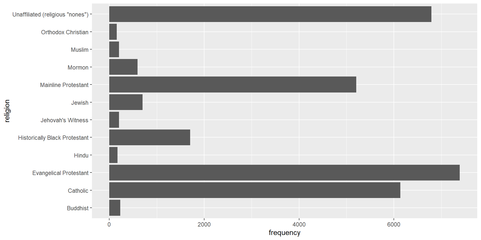
ggplot(rel_inc_long, aes(y = religion, x = frequency)) +geom_col()
The religion names are long. On the x-axis they’d overlap, so the categorical variable goes on the y-axis where the names read like regular text. We use geom_col() instead of geom_bar(). geom_bar() counts the rows for us, but these data are already a summary table with the frequencies calculated. geom_col() uses the x value we give it for the length of each bar.
Recode religion
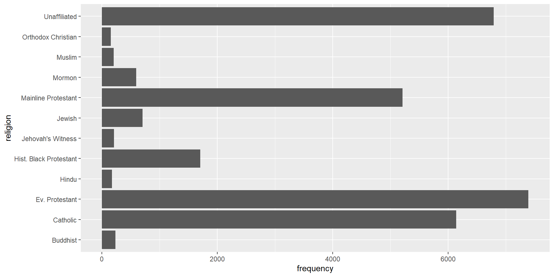
rel_inc_long <- rel_inc_long %>%mutate(religion =case_when( religion =="Evangelical Protestant"~"Ev. Protestant", religion =="Historically Black Protestant"~"Hist. Black Protestant", religion =='Unaffiliated (religious "nones")'~"Unaffiliated",TRUE~ religion))
Recode religion, explained
Some religion names are much longer than others, which makes the plot harder to read. We replace a few of them with shorter strings using case_when() inside mutate(). We overwrite the existing religion variable. Each condition on the left is a case, and when it’s true, we get the value on the right.
'Unaffiliated (religious "nones")' already has double quotes inside it, so we wrap it in single quotes. Otherwise the two strings get mixed up. The style guide recommends double quotes, so that’s what we use everywhere else.
TRUE ~ religion catches everything else. If none of the first three conditions are true, we keep the old value of religion.
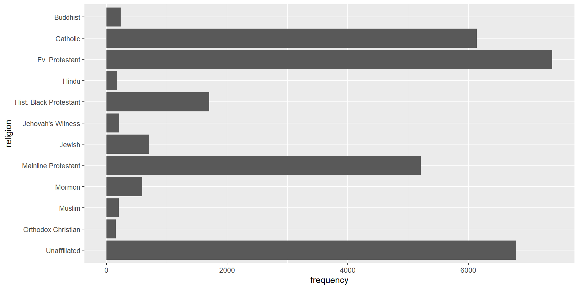
Before, the plot read Buddhist, Catholic, Evangelical Protestant going up the y-axis, which seems odd. fct_rev() from forcats (the fct_ prefix) reverses the order of the levels, so we don’t have to write them all out. Now the plot reads alphabetically from top to bottom.
Add income
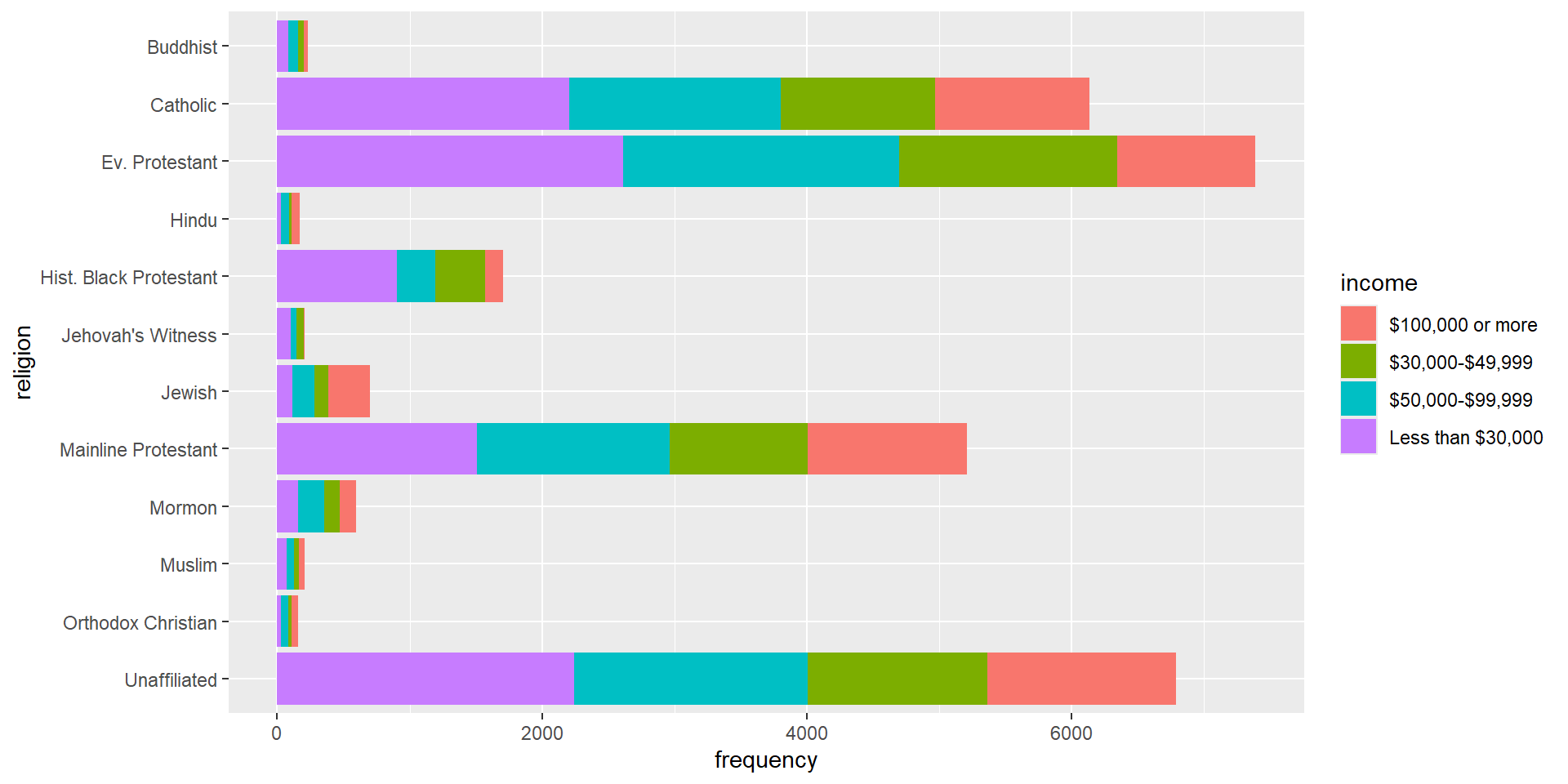
ggplot(rel_inc_long, aes(y = religion, x = frequency, fill = income)) +geom_col()
Filling the bars by income gives a segmented bar plot. Is the income distribution different across religious traditions? That’s hard to answer here. Some traditions are much more common than others, so their bars are much longer and the counts aren’t comparable.
Fill bars
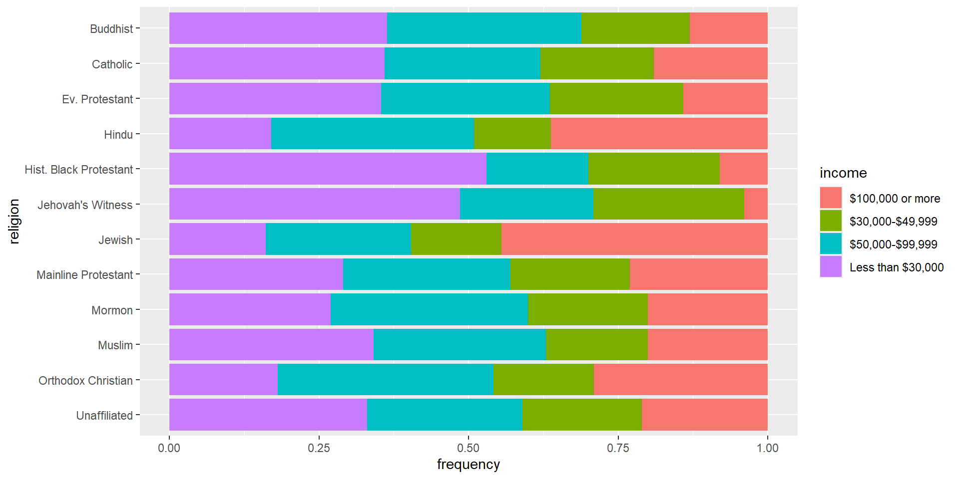
ggplot(rel_inc_long, aes(y = religion, x = frequency, fill = income)) +geom_col(position ="fill")
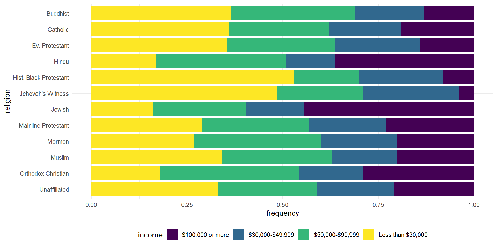
position = "fill" stretches every bar to a length of 1. The segments now show proportions instead of frequencies, so we’ve come full circle. Now we can compare. The proportion making less than $30,000 is about the same for Buddhist, Catholic, and Evangelical Protestant groups. It’s much higher for Historically Black Protestant and Jehovah’s Witness groups.
Change colors
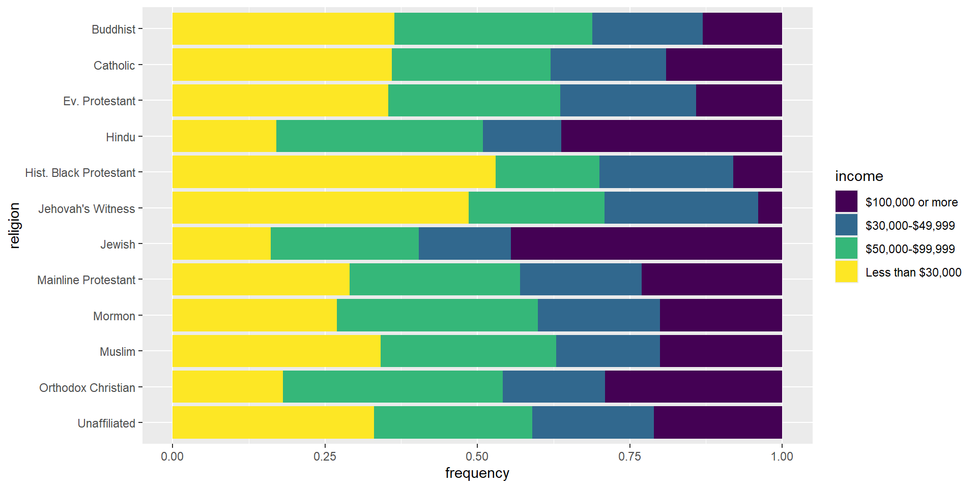
ggplot(rel_inc_long, aes(y = religion, x = frequency, fill = income)) +geom_col(position ="fill") +scale_fill_viridis_d()
We switch from the default ggplot2 colors to the viridis scale. We’re changing the colors of the fill aesthetic, so the function is scale_fill_viridis_d(). The _d stands for discrete, as opposed to continuous.
Change theme
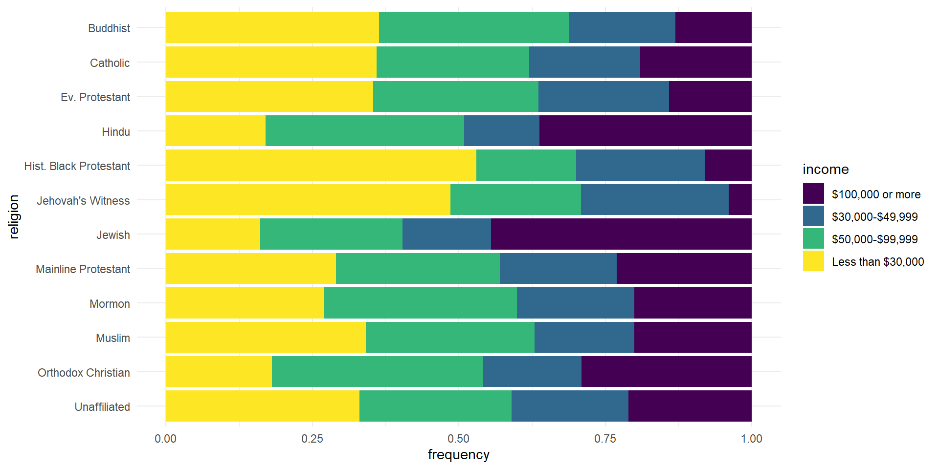
ggplot(rel_inc_long, aes(y = religion, x = frequency, fill = income)) +geom_col(position ="fill") +scale_fill_viridis_d() +theme_minimal()
The default ggplot2 theme is theme_gray(), and the gray box behind the bars looks a little busy. theme_minimal() cleans it up. It’s added as another layer.
Move legend to the bottom
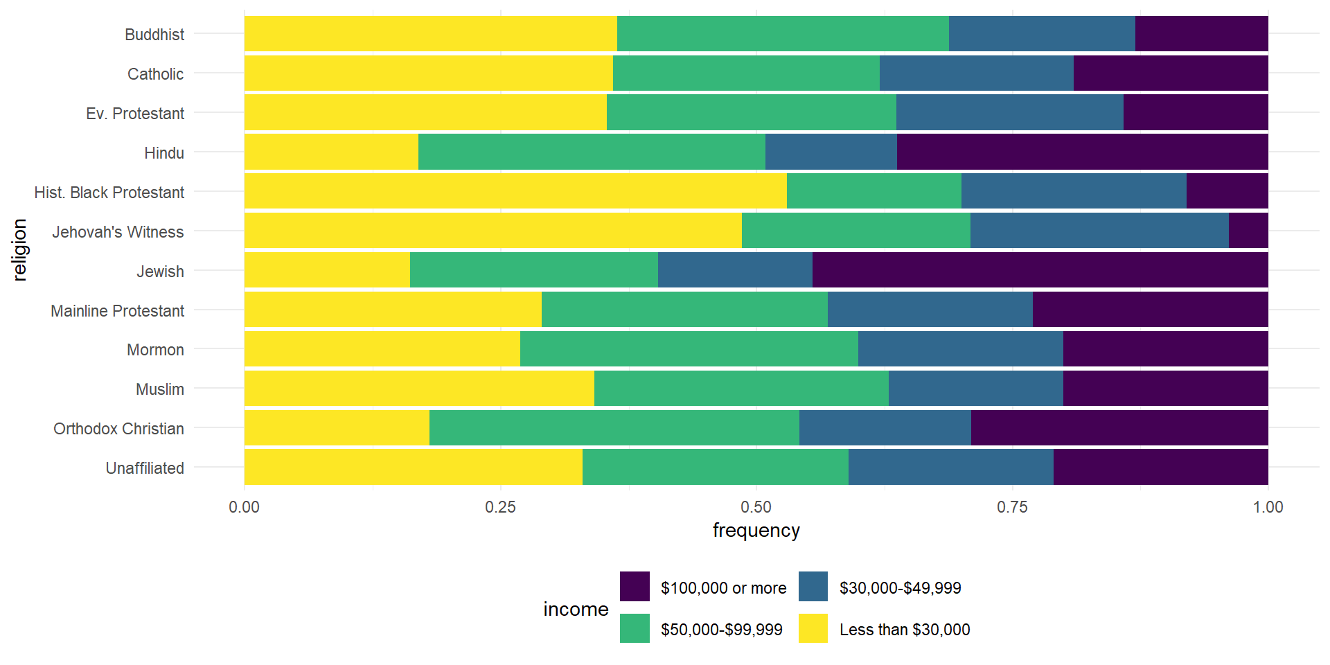
ggplot(rel_inc_long, aes(y = religion, x = frequency, fill = income)) +geom_col(position ="fill") +scale_fill_viridis_d() +theme_minimal() +theme(legend.position ="bottom")
Moving the legend to the bottom gives the plot more room. We do it in the theme() layer. You aren’t expected to know customizations like this by heart. Look them up in the help file, and sometimes just try them to see what you get.
The legend was spread across one row. The guides() layer puts the legend for the fill aesthetic into two rows, filled in by row, so it’s more compact.
Fix labels
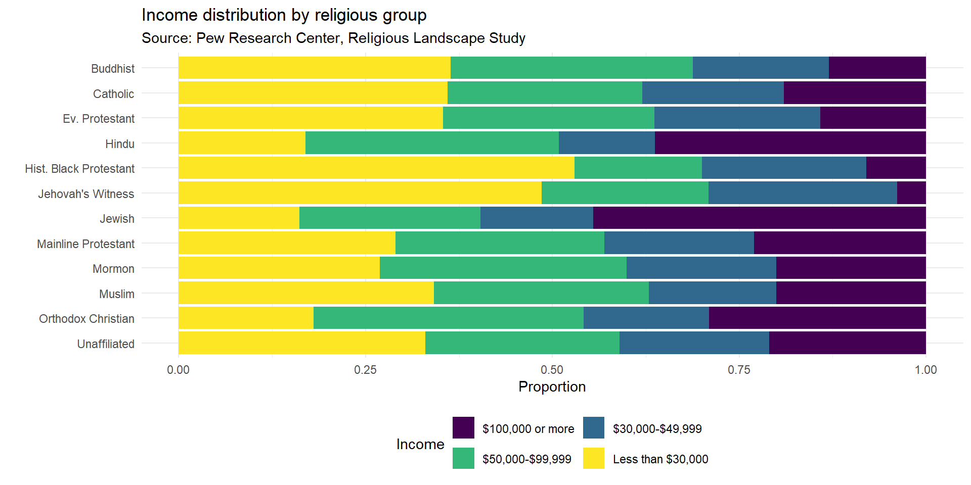
ggplot(rel_inc_long, aes(y = religion, x = frequency, fill = income)) +geom_col(position ="fill") +scale_fill_viridis_d() +theme_minimal() +theme(legend.position ="bottom") +guides(fill =guide_legend(nrow =2, byrow =TRUE)) +labs(x ="Proportion", y ="", title ="Income distribution by religious group",subtitle ="Source: Pew Research Center, Religious Landscape Study",fill ="Income")
In labs() we drop the y label, add an informative title, cite the source, and relabel the x-axis and the legend.
Recap
We started with a plot that wasn’t very informative, mostly because some religious groups had much bigger sample sizes than others. Step by step, we got to a plot where we can compare income levels across religious traditions. We can see which traditions have the highest proportions at lower incomes, and which have more people in the higher brackets.
Could we keep improving it? Sure. The point is that the functions for reading data, working with factors, and customizing plots start to feel like useful tools once you use them together.
Acknowledgements & Credits
Note
This page adapts material from Data Science in a Box (Unit 2, Deck 13: “Recoding data”) by Mine Çetinkaya-Rundel, licensed under CC BY-SA 4.0. Source: tidyverse/datascience-box. Modified: converted from xaringan to Quarto revealjs; added talking points from the DSBox video.