wk6-d02-reshaping
Chico State
DATA 385 - Fall 2026
September 30, 2026
🎥wk6-d02 reshaping
We have data organized in an unideal way for our analysis. We want to reorganize the data to carry on with our analysis. This isn’t messy data. It has all the information we need, just not in the shape we need it.
# A tibble: 2 × 4
customer_id item_1 item_2 item_3
<dbl> <chr> <chr> <chr>
1 1 bread milk banana
2 2 milk toilet paper <NA>
# A tibble: 6 × 3
customer_id item_no item
<dbl> <chr> <chr>
1 1 item_1 bread
2 1 item_2 milk
3 1 item_3 banana
4 2 item_1 milk
5 2 item_2 toilet paper
6 2 item_3 <NA>
Back to the grocery sales from d01. We have one row per customer, with a column for each item they bought: customer 1 bought bread, milk, and a banana; customer 2 only bought milk and toilet paper, so their third item is NA. We want one row per customer per item, the format we used for further analysis in d01.

The goal of tidyr is to help you tidy your data via
NAs should be treatedIf you’ve ever seen Friends, this is what “pivot” brings to mind. That’s not what we’re talking about.
Taking data from wider to longer, and back.
more columns
# A tibble: 2 × 4
customer_id item_1 item_2 item_3
<dbl> <chr> <chr> <chr>
1 1 bread milk banana
2 2 milk toilet paper <NA>
more rows
# A tibble: 6 × 3
customer_id item_no item
<dbl> <chr> <chr>
1 1 item_1 bread
2 1 item_2 milk
3 1 item_3 banana
4 2 item_1 milk
5 2 item_2 toilet paper
6 2 item_3 <NA>
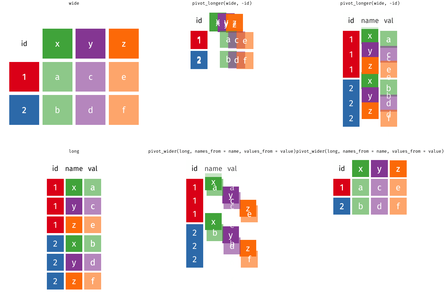
Try not to say “wide” or “long”. The same data frame might be either, depending on what you want to do next. Instead ask: are we making it wider (adding columns) or longer (adding rows)? The clipboard person writing each customer’s items across columns created a wider data frame; here we want to go from wider to longer.
pivot_longer()data (as usual)cols: columns to pivot into longer formatnames_to: name of the column where column names of pivoted variables go (character string)values_to: name of the column where data in pivoted variables go (character string)Like every other tidyverse function, the first argument is the data. names_to and values_to are two new variables that don’t exist in the original data frame yet, which is why we give their names as character strings. They go in quotes.
# A tibble: 6 × 3
customer_id item_no item
<dbl> <chr> <chr>
1 1 item_1 bread
2 1 item_2 milk
3 1 item_3 banana
4 2 item_1 milk
5 2 item_2 toilet paper
6 2 item_3 <NA>
The columns we pivot are the ones with the items the customers bought, item_1 through item_3, picked with the colon operator. The column names go into a new column called item_no, the values in the cells go into a new column called item, and we end up with 6 rows and 3 columns.
Most likely, because the next step of your analysis needs it
Now that there’s one row per item purchased, we can join the prices and go on to calculate things like total revenue.
data (as usual)names_from: which column in the long format contains the what should be column names in the wide formatvalues_from: which column in the long format contains the what should be values in the new columns in the wide formatNote that item_no and item are not quoted here: they’re variables that already exist in the data frame, so we’re just saying where to grab information from, rather than naming new variables.
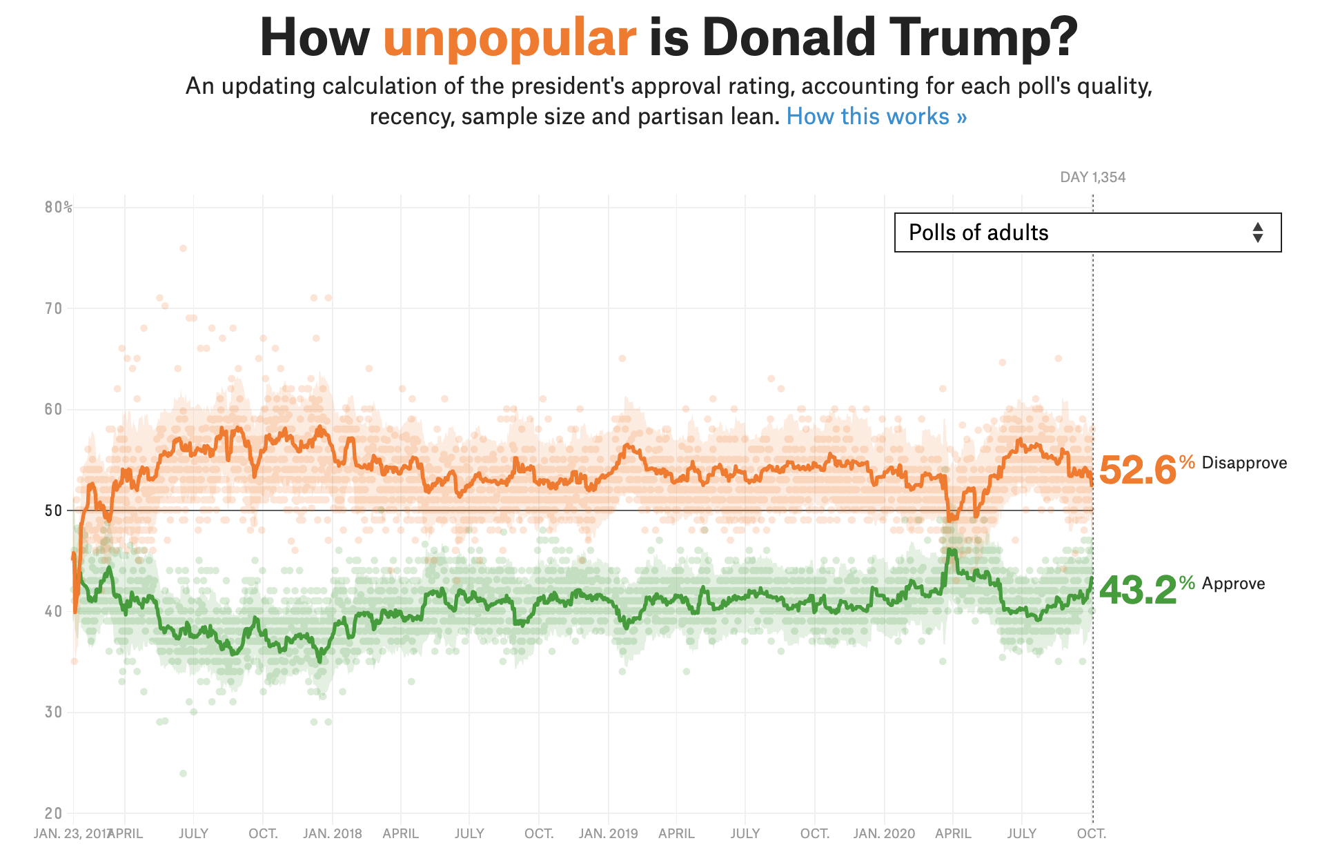
Source: FiveThirtyEight
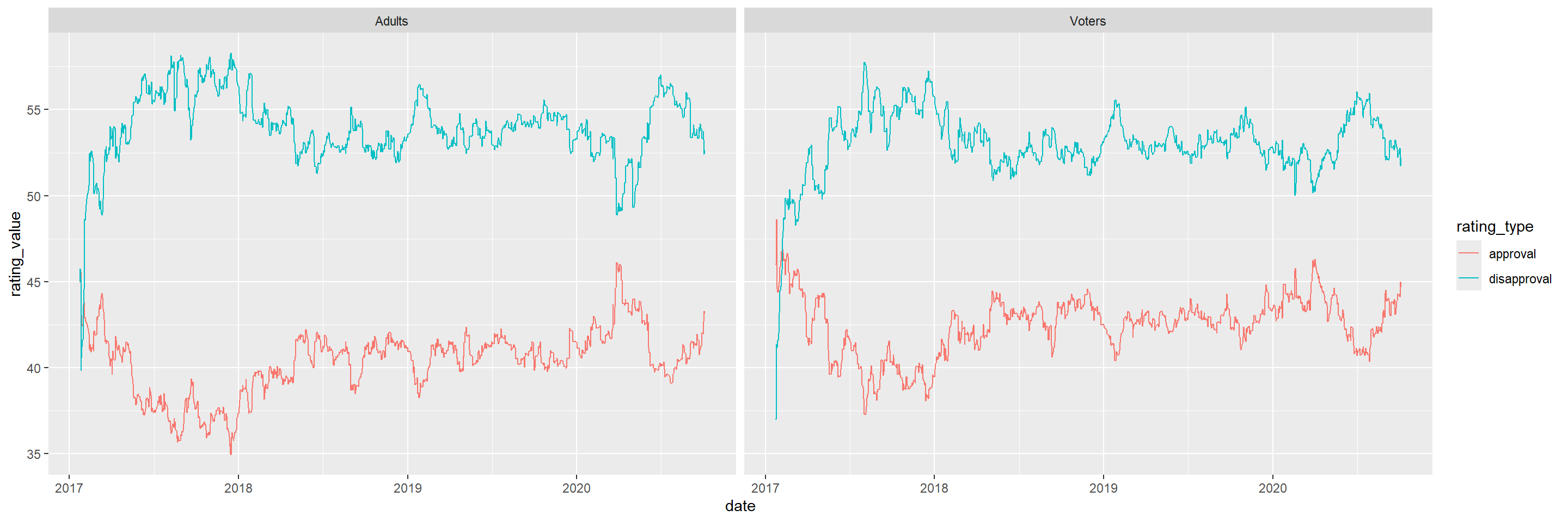
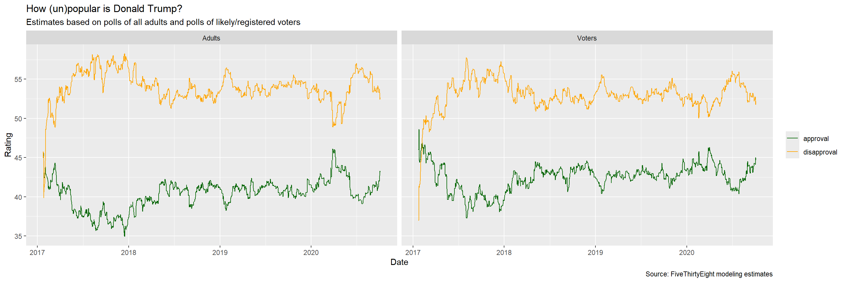
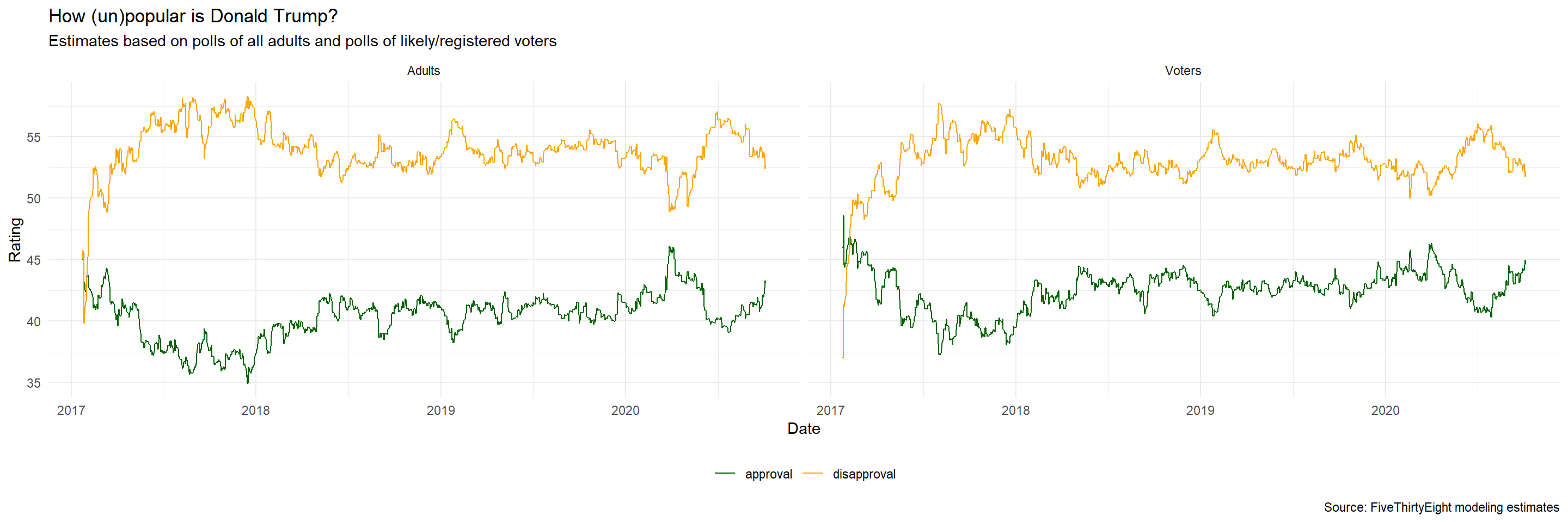
FiveThirtyEight aggregated polls with models to estimate approval (green) and disapproval (orange) over the whole presidency. We won’t do the modeling. We take their model results as given and recreate a static version of this plot, for polls of all adults and polls of likely/registered voters.
# A tibble: 2,702 × 4
subgroup date approval disapproval
<chr> <date> <dbl> <dbl>
1 Voters 2020-10-04 44.7 52.2
2 Adults 2020-10-04 43.2 52.6
3 Adults 2020-10-03 43.2 52.6
4 Voters 2020-10-03 45.0 51.7
5 Adults 2020-10-02 43.3 52.4
6 Voters 2020-10-02 44.5 52.1
7 Voters 2020-10-01 44.1 52.8
8 Adults 2020-10-01 42.7 53.3
9 Adults 2020-09-30 42.2 53.7
10 Voters 2020-09-30 44.2 52.7
# ℹ 2,692 more rows
Downloaded from FiveThirtyEight and lightly cleaned. subgroup is either Voters or Adults, so there are two rows per date. approval and disapproval are model estimates, not ground truth. E.g. as of October 4, the estimate for likely voters is 44.7% approval and 52.2% disapproval.

Aesthetic mappings:
✅ x = date
❌ y = rating_value
❌ color = rating_type
Facet: ✅ subgroup (Adults and Voters)
What pieces go into this plot? date and subgroup are already in the data. But the rating is spread across two columns, approval and disapproval, and ggplot needs whatever goes on an axis in a single variable. So we need two new variables: rating_value (currently in the cells) and rating_type (currently in the column headers).
# A tibble: 6 × 4
subgroup date rating_type rating_value
<chr> <date> <chr> <dbl>
1 Voters 2020-10-04 approval 44.7
2 Voters 2020-10-04 disapproval 52.2
3 Adults 2020-10-04 approval 43.2
4 Adults 2020-10-04 disapproval 52.6
5 Adults 2020-10-03 approval 43.2
6 Adults 2020-10-03 disapproval 52.6
The columns we pivot are approval and disapproval. Their names go into a new variable rating_type, and their values into a new variable rating_value.
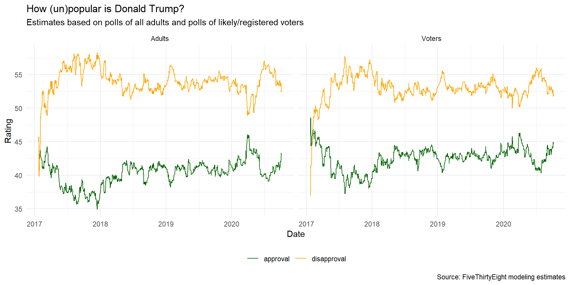
date on the x-axis, rating_value on the y-axis, color by rating_type, facet by subgroup. geom_line() joins the points with lines, and the group aesthetic tells it which points to join. We want one line for approval and one for disapproval.
ggplot(trump_longer,
aes(x = date, y = rating_value, color = rating_type, group = rating_type)) +
geom_line() + facet_wrap(~ subgroup) +
scale_color_manual(values = c("darkgreen", "orange")) + # hand color lines
labs(
x = "Date", y = "Rating",
color = NULL, # drop legend title
title = "How (un)popular is Donald Trump?",
subtitle = "Estimates based on polls of all adults and polls of likely/registered voters",
caption = "Source: FiveThirtyEight modeling estimates")ggplot(trump_longer,
aes(x = date, y = rating_value, color = rating_type, group = rating_type)) +
geom_line() + facet_wrap(~ subgroup) +
scale_color_manual(values = c("darkgreen", "orange")) +
labs(
x = "Date", y = "Rating",
color = NULL,
title = "How (un)popular is Donald Trump?",
subtitle = "Estimates based on polls of all adults and polls of likely/registered voters",
caption = "Source: FiveThirtyEight modeling estimates") +
theme_minimal() + # get rid of gray background
theme(legend.position = "bottom") # moves the legend so it takes up less spaceIn this case study we started with data that had the information we needed, but not in the shape we wanted. First we reorganized it into a shape that’s easy to plot with ggplot2, then we made cosmetic adjustments to make the plot more visually appealing.
Note
This page adapts material from Data Science in a Box (Unit 2, Deck 9: “Tidying data”) by Mine Çetinkaya-Rundel, licensed under CC BY-SA 4.0. Source: tidyverse/datascience-box. Modified: converted from xaringan to Quarto revealjs; added some talking points from the DSBox video.