Working with multiple data frames

wk6-d01-multi-df

Dr. D

Chico State
DATA 385 - Fall 2026

September 29, 2026

Setup

🎥wk6-d01 multiple df

library(tidyverse)

So far we’ve worked with a single data frame and transformed it with dplyr functions. Now we have multiple data frames, and we want to bring them together.

Data: Women in science

professions <- read_csv(here::here("notes/data/professions.csv"))
dates <- read_csv(here::here("notes/data/dates.csv"))
works <- read_csv(here::here("notes/data/works.csv"))

name
Ada Lovelace
Marie Curie
Janaki Ammal
Chien-Shiung Wu
Katherine Johnson
Rosalind Franklin
Vera Rubin
Gladys West
Flossie Wong-Staal
Jennifer Doudna

The information on these 10 scientists has been spread across three data frames on purpose. Not every data frame has information on every scientist, which is a lot closer to real life than having complete data on everyone.
Source: Discover Magazine

Inputs: `professions`

professions

# A tibble: 10 × 2
   name               profession                        
   <chr>              <chr>                             
 1 Ada Lovelace       Mathematician                     
 2 Marie Curie        Physicist and Chemist             
 3 Janaki Ammal       Botanist                          
 4 Chien-Shiung Wu    Physicist                         
 5 Katherine Johnson  Mathematician                     
 6 Rosalind Franklin  Chemist                           
 7 Vera Rubin         Astronomer                        
 8 Gladys West        Mathematician                     
 9 Flossie Wong-Staal Virologist and Molecular Biologist
10 Jennifer Doudna    Biochemist

We know the profession of all 10 scientists. e.g. Ada Lovelace was a mathematician, Marie Curie a physicist and chemist. This is the only complete data frame.

Inputs: `dates`

dates

# A tibble: 8 × 3
  name               birth_year death_year
  <chr>                   <dbl>      <dbl>
1 Janaki Ammal             1897       1984
2 Chien-Shiung Wu          1912       1997
3 Katherine Johnson        1918       2020
4 Rosalind Franklin        1920       1958
5 Vera Rubin               1928       2016
6 Gladys West              1930         NA
7 Flossie Wong-Staal       1947         NA
8 Jennifer Doudna          1964         NA

We have birth and death years for 8 of the 10 scientists. An NA for death_year doesn’t mean unknown, but that she is still living.

Inputs: `works`

works

# A tibble: 9 × 2
  name               known_for                                        
  <chr>              <chr>                                            
1 Ada Lovelace       first computer algorithm                         
2 Marie Curie        theory of radioactivity,  discovery of elements …
3 Janaki Ammal       hybrid species, biodiversity protection          
4 Chien-Shiung Wu    confim and refine theory of radioactive beta dec…
5 Katherine Johnson  calculations of orbital mechanics critical to se…
6 Vera Rubin         existence of dark matter                         
7 Gladys West        mathematical modeling of the shape of the Earth …
8 Flossie Wong-Staal first scientist to clone HIV and create a map of…
9 Jennifer Doudna    one of the primary developers of CRISPR, a groun…

For 9 of the 10 scientists we have information on what they’re known for e.g. Ada Lovelace for the first computer algorithm, Marie Curie for the theory of radioactivity.

Desired output

# A tibble: 10 × 5
   name               profession       birth_year death_year known_for
   <chr>              <chr>                 <dbl>      <dbl> <chr>    
 1 Ada Lovelace       Mathematician            NA         NA first co…
 2 Marie Curie        Physicist and C…         NA         NA theory o…
 3 Janaki Ammal       Botanist               1897       1984 hybrid s…
 4 Chien-Shiung Wu    Physicist              1912       1997 confim a…
 5 Katherine Johnson  Mathematician          1918       2020 calculat…
 6 Rosalind Franklin  Chemist                1920       1958 <NA>     
 7 Vera Rubin         Astronomer             1928       2016 existenc…
 8 Gladys West        Mathematician          1930         NA mathemat…
 9 Flossie Wong-Staal Virologist and …       1947         NA first sc…
10 Jennifer Doudna    Biochemist             1964         NA one of t…

One row per scientist (10 rows) and 5 columns: name, profession from the first data frame, birth_year and death_year from the second, and known_for from the third.

Inputs, reminder

names(professions)

[1] "name"       "profession"

names(dates)

[1] "name"       "birth_year" "death_year"

names(works)

[1] "name"      "known_for"

nrow(professions)

[1] 10

nrow(dates)

[1] 8

nrow(works)

[1] 9

All three share one variable, name, and that’s what gets used as the linking variable by default. We know they don’t all have the same number of rows, but we don’t yet know which scientists are missing from which data frame.

Joining data frames

something_join(x, y)

left_join(): all rows from x
right_join(): all rows from y
full_join(): all rows from both x and y
semi_join(): all rows from x where there are matching values in y, keeping just columns from x
inner_join(): all rows from x where there are matching values in y, return all combination of multiple matches in the case of multiple matches
anti_join(): return all rows from x where there are not matching values in y, never duplicate rows of x
… and more

Example data frames `x` and `y`

For the next few slides…

(x <- tibble(
  id = c(1, 2, 3),
  value_x = c("x1", "x2", "x3")))

# A tibble: 3 × 2
     id value_x
  <dbl> <chr>  
1     1 x1     
2     2 x2     
3     3 x3

(y <- tibble(
  id = c(1, 2, 4),
  value_y = c("y1", "y2", "y4")))

# A tibble: 3 × 2
     id value_y
  <dbl> <chr>  
1     1 y1     
2     2 y2     
3     4 y4

Some ids are in both data frames (1 and 2) and some are in only one (3 and 4), so it’s easy to see what each join keeps.

`left_join()`

left_join(x, y)

# A tibble: 3 × 3
     id value_x value_y
  <dbl> <chr>   <chr>  
1     1 x1      y1     
2     2 x2      y2     
3     3 x3      <NA>

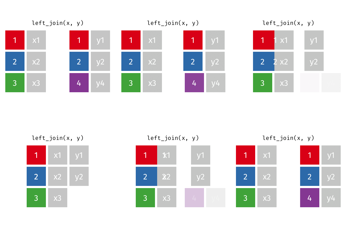
Keep all the rows of x (the left one), and bring along the information from y wherever it exists. id = 4 exists in y but not in x, so it disappears.

`left_join()`

professions %>%
  left_join(dates)

# A tibble: 10 × 4
   name               profession                 birth_year death_year
   <chr>              <chr>                           <dbl>      <dbl>
 1 Ada Lovelace       Mathematician                      NA         NA
 2 Marie Curie        Physicist and Chemist              NA         NA
 3 Janaki Ammal       Botanist                         1897       1984
 4 Chien-Shiung Wu    Physicist                        1912       1997
 5 Katherine Johnson  Mathematician                    1918       2020
 6 Rosalind Franklin  Chemist                          1920       1958
 7 Vera Rubin         Astronomer                       1928       2016
 8 Gladys West        Mathematician                    1930         NA
 9 Flossie Wong-Staal Virologist and Molecular …       1947         NA
10 Jennifer Doudna    Biochemist                       1964         NA

We keep all the information from professions and bring in birth_year and death_year. Ada Lovelace and Marie Curie are missing from dates, so they get NA birth and death years. we don’t lose their rows, because they exist in professions.

`right_join()`

right_join(x, y)

# A tibble: 3 × 3
     id value_x value_y
  <dbl> <chr>   <chr>  
1     1 x1      y1     
2     2 x2      y2     
3     4 <NA>    y4

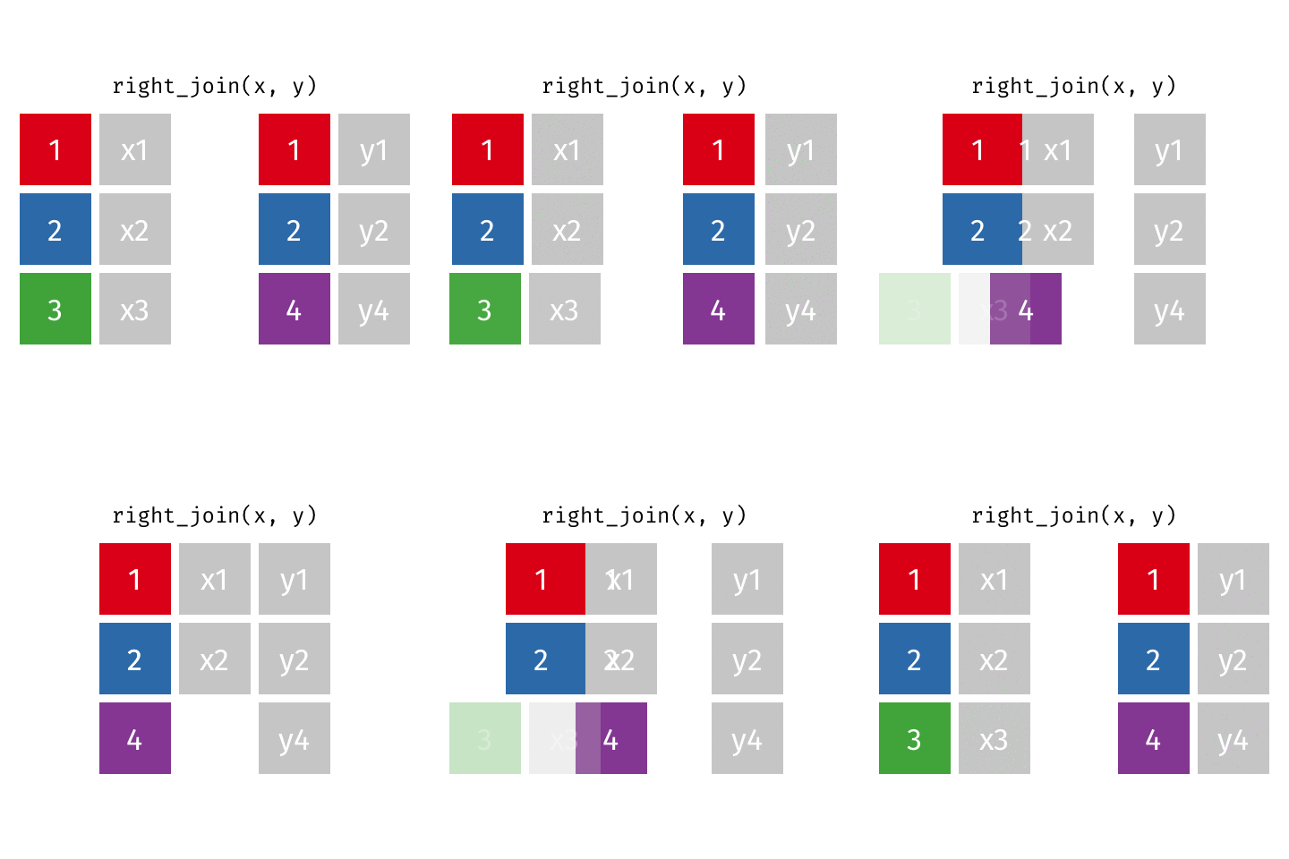
The same thing the other way around: keep all the rows of y, and id 3 goes away.

❓Why not just swap the order in a left_join()?

`right_join()`

professions %>%
  right_join(dates)

# A tibble: 8 × 4
  name               profession                  birth_year death_year
  <chr>              <chr>                            <dbl>      <dbl>
1 Janaki Ammal       Botanist                          1897       1984
2 Chien-Shiung Wu    Physicist                         1912       1997
3 Katherine Johnson  Mathematician                     1918       2020
4 Rosalind Franklin  Chemist                           1920       1958
5 Vera Rubin         Astronomer                        1928       2016
6 Gladys West        Mathematician                     1930         NA
7 Flossie Wong-Staal Virologist and Molecular B…       1947         NA
8 Jennifer Doudna    Biochemist                        1964         NA

This time we lose Ada Lovelace and Marie Curie, since they aren’t in dates. Everyone else gets their profession from professions.

`full_join()`

full_join(x, y)

# A tibble: 4 × 3
     id value_x value_y
  <dbl> <chr>   <chr>  
1     1 x1      y1     
2     2 x2      y2     
3     3 x3      <NA>   
4     4 <NA>    y4

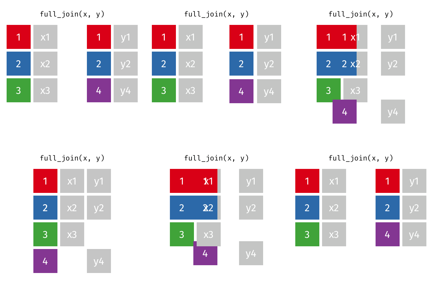
Keep all the rows from both, and wherever information is missing we end up with NAs.

`full_join()`

dates %>%
  full_join(works)

# A tibble: 10 × 4
   name               birth_year death_year known_for                 
   <chr>                   <dbl>      <dbl> <chr>                     
 1 Janaki Ammal             1897       1984 hybrid species, biodivers…
 2 Chien-Shiung Wu          1912       1997 confim and refine theory …
 3 Katherine Johnson        1918       2020 calculations of orbital m…
 4 Rosalind Franklin        1920       1958 <NA>                      
 5 Vera Rubin               1928       2016 existence of dark matter  
 6 Gladys West              1930         NA mathematical modeling of …
 7 Flossie Wong-Staal       1947         NA first scientist to clone …
 8 Jennifer Doudna          1964         NA one of the primary develo…
 9 Ada Lovelace               NA         NA first computer algorithm  
10 Marie Curie                NA         NA theory of radioactivity, …

dates has 8 scientists and works has 9, but not the same ones. We get dates for the 8, and known_for for Ada Lovelace and Marie Curie from works. Rosalind Franklin is missing from works, so her known_for is NA. We end up with all 10 rows because we had at least one piece of information about all 10 women.

`inner_join()`

inner_join(x, y)

# A tibble: 2 × 3
     id value_x value_y
  <dbl> <chr>   <chr>  
1     1 x1      y1     
2     2 x2      y2

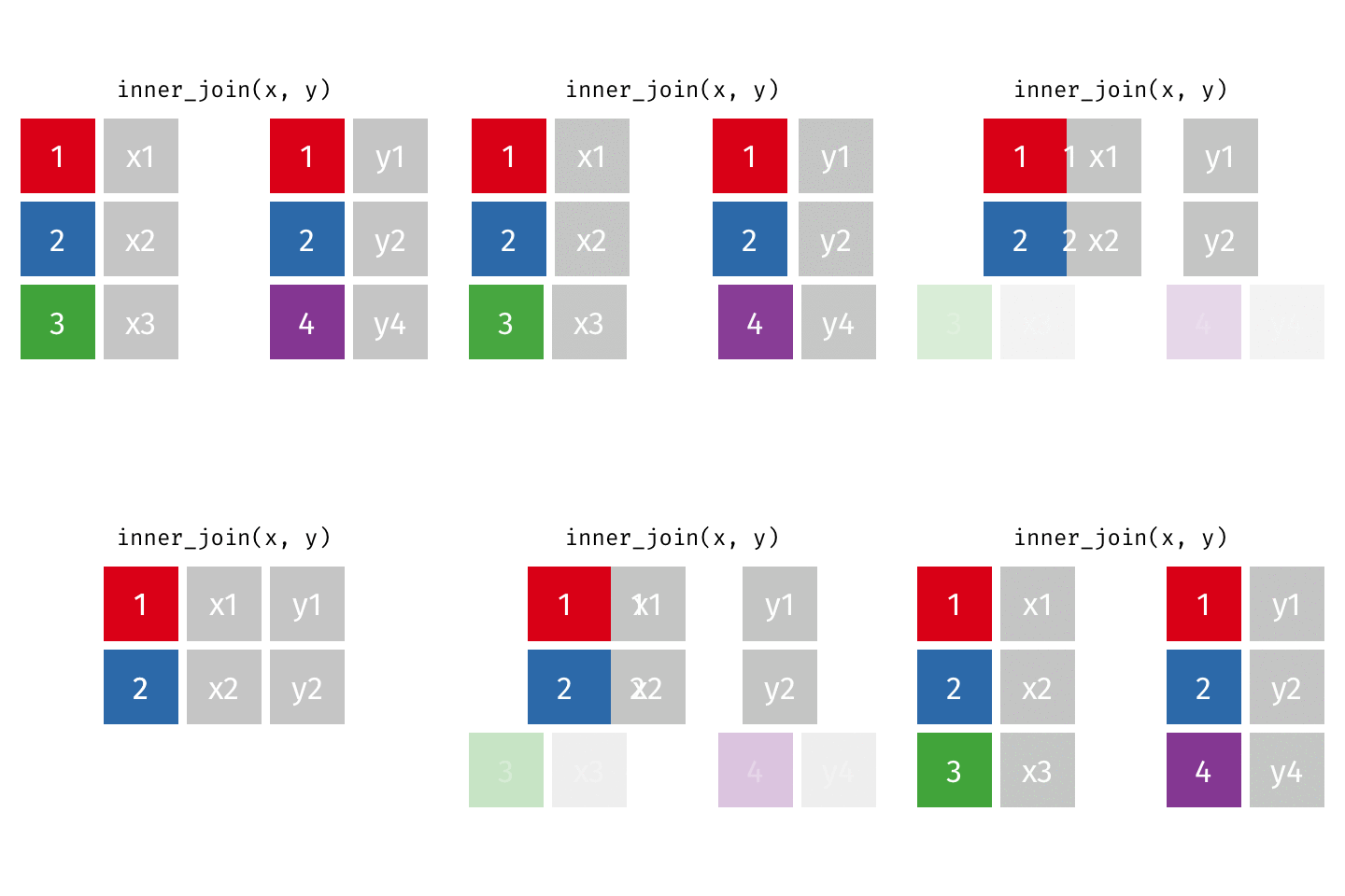
An intersection: only give me the rows for which I have data in both data frames.

`inner_join()`

dates %>%
  inner_join(works)

# A tibble: 7 × 4
  name               birth_year death_year known_for                  
  <chr>                   <dbl>      <dbl> <chr>                      
1 Janaki Ammal             1897       1984 hybrid species, biodiversi…
2 Chien-Shiung Wu          1912       1997 confim and refine theory o…
3 Katherine Johnson        1918       2020 calculations of orbital me…
4 Vera Rubin               1928       2016 existence of dark matter   
5 Gladys West              1930         NA mathematical modeling of t…
6 Flossie Wong-Staal       1947         NA first scientist to clone H…
7 Jennifer Doudna          1964         NA one of the primary develop…

Only the 7 scientists that are in both dates and works.

`semi_join()`

semi_join(x, y)

# A tibble: 2 × 2
     id value_x
  <dbl> <chr>  
1     1 x1     
2     2 x2

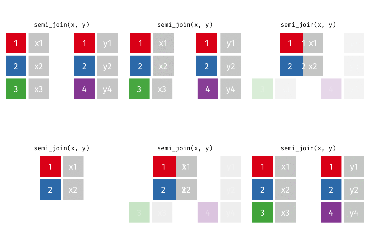
Very similar to an inner join, except the information in y is only used to decide which rows of x to keep. None of y’s columns come along.

`semi_join()`

dates %>%
  semi_join(works)

# A tibble: 7 × 3
  name               birth_year death_year
  <chr>                   <dbl>      <dbl>
1 Janaki Ammal             1897       1984
2 Chien-Shiung Wu          1912       1997
3 Katherine Johnson        1918       2020
4 Vera Rubin               1928       2016
5 Gladys West              1930         NA
6 Flossie Wong-Staal       1947         NA
7 Jennifer Doudna          1964         NA

The same 7 rows as the inner join, but there’s no known_for column. That column is gone.

`anti_join()`

anti_join(x, y)

# A tibble: 1 × 2
     id value_x
  <dbl> <chr>  
1     3 x3

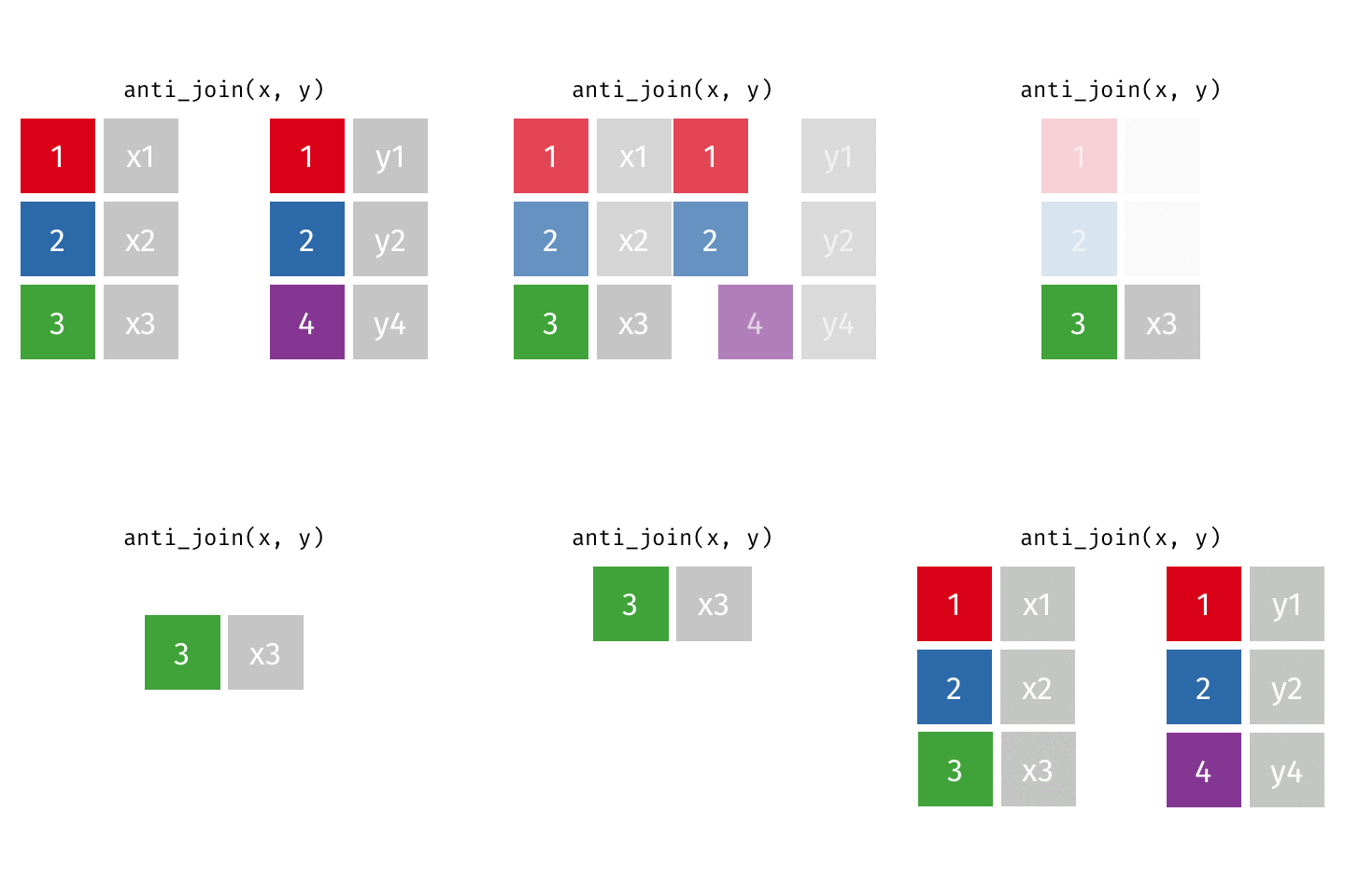
A subtraction: the rows in x that are not in y.

`anti_join()`

dates %>%
  anti_join(works)

# A tibble: 1 × 3
  name              birth_year death_year
  <chr>                  <dbl>      <dbl>
1 Rosalind Franklin       1920       1958

The one scientist we have birth and death years for, but no information on what she’s known for: Rosalind Franklin.

Putting it altogether

professions %>%
  left_join(dates) %>%
  left_join(works)

# A tibble: 10 × 5
   name               profession       birth_year death_year known_for
   <chr>              <chr>                 <dbl>      <dbl> <chr>    
 1 Ada Lovelace       Mathematician            NA         NA first co…
 2 Marie Curie        Physicist and C…         NA         NA theory o…
 3 Janaki Ammal       Botanist               1897       1984 hybrid s…
 4 Chien-Shiung Wu    Physicist              1912       1997 confim a…
 5 Katherine Johnson  Mathematician          1918       2020 calculat…
 6 Rosalind Franklin  Chemist                1920       1958 <NA>     
 7 Vera Rubin         Astronomer             1928       2016 existenc…
 8 Gladys West        Mathematician          1930         NA mathemat…
 9 Flossie Wong-Staal Virologist and …       1947         NA first sc…
10 Jennifer Doudna    Biochemist             1964         NA one of t…

Start with professions because it has all 10 rows. Left join dates to get birth and death years for whoever we have them for (still 10 rows), then left join works to get known_for.

We never had to say “match by name” because it’s the only column the three have in common. It had to be spelled exactly the same way in all of them for this to work.

Case study: Student records

Student records

Have:
- Enrollment: official university enrollment records
- Survey: Student provided info missing students who never filled it out and including students who filled it out but dropped the class
Want: Survey info for all enrolled in class

enrolment <- read_csv(here::here("notes/data/enrolment.csv"))
survey <- read_csv(here::here("notes/data/survey.csv"))

enrolment

# A tibble: 3 × 2
     id name           
  <dbl> <chr>          
1     1 Dave Friday    
2     2 Hermine        
3     3 Sura Selvarajah

survey

# A tibble: 4 × 3
     id name    username            
  <dbl> <chr>   <chr>               
1     2 Hermine bakealongwithhermine
2     3 Sura    surasbakes          
3     4 Peter   peter_bakes         
4     5 Mark    thebakingbuddha

Student records: in class

enrolment %>%
  left_join(survey, by = "id")

# A tibble: 3 × 4
     id name.x          name.y  username            
  <dbl> <chr>           <chr>   <chr>               
1     1 Dave Friday     <NA>    <NA>                
2     2 Hermine         Hermine bakealongwithhermine
3     3 Sura Selvarajah Sura    surasbakes

Start with enrolment, since the official records are the truth on any given day. Use the by argument, with the column name as a character string, to say “don’t try to match by name, just match by id.” Both data frames had a name column, so R keeps both and adds the suffixes .x (first data frame) and .y (second data frame).

Student records: survey missing

enrolment %>%
  anti_join(survey, by = "id")

# A tibble: 1 × 2
     id name       
  <dbl> <chr>      
1     1 Dave Friday

In enrolment but not in survey. Chase these students down for their survey.

Student records: dropped

survey %>%
  anti_join(enrolment, by = "id")

# A tibble: 2 × 3
     id name  username       
  <dbl> <chr> <chr>          
1     4 Peter peter_bakes    
2     5 Mark  thebakingbuddha

Filled out the survey in the first days of class, but no longer on the enrollment records. Don’t need, dropped from further records (e.g. removed from the class GitHub organization).

Case study: Grocery sales

Grocery sales

Have:
- Purchases: One row per customer per item (purchases)
- Prices: One row per item in the store, listing their prices
Want: Total revenue

purchases <- read_csv(here::here("notes/data/purchases.csv"))
prices <- read_csv(here::here("notes/data/prices.csv"))

purchases

# A tibble: 5 × 2
  customer_id item        
        <dbl> <chr>       
1           1 bread       
2           1 milk        
3           1 banana      
4           2 milk        
5           2 toilet paper

prices

# A tibble: 5 × 2
  item         price
  <chr>        <dbl>
1 avocado       0.5 
2 banana        0.15
3 bread         1   
4 milk          0.8 
5 toilet paper  3

Grocery sales: total revenue

purchases %>%
  left_join(prices)

# A tibble: 5 × 3
  customer_id item         price
        <dbl> <chr>        <dbl>
1           1 bread         1   
2           1 milk          0.8 
3           1 banana        0.15
4           2 milk          0.8 
5           2 toilet paper  3

purchases %>%
  left_join(prices) %>%
  summarise(total_revenue = sum(price))

# A tibble: 1 × 1
  total_revenue
          <dbl>
1          5.75

Start with purchases and left join prices to see the price of each item purchased. Once the data are in a single data frame, the single data frame verbs work as usual: sum up the price column for a total revenue of £5.75.

Grocery sales: revenue per customer

purchases %>%
  left_join(prices)

# A tibble: 5 × 3
  customer_id item         price
        <dbl> <chr>        <dbl>
1           1 bread         1   
2           1 milk          0.8 
3           1 banana        0.15
4           2 milk          0.8 
5           2 toilet paper  3

purchases %>%
  left_join(prices) %>%
  group_by(customer_id) %>%
  summarise(total_revenue = sum(price))

# A tibble: 2 × 2
  customer_id total_revenue
        <dbl>         <dbl>
1           1          1.95
2           2          3.8

All it takes is a group_by() right before the summarise().

In both case studies the data lived in separate data frames, and we had to bring them together first before we could get any further insight from them.

Acknowledgements & Credits

Note

This page adapts material from Data Science in a Box (Unit 2, Deck 8: “Working with multiple data frames”) by Mine Çetinkaya-Rundel, licensed under CC BY-SA 4.0. Source: tidyverse/datascience-box. Modified: converted from xaringan to Quarto revealjs; added talking points from the DSBox video.

Working with multiple data frames

Setup

Data: Women in science

Inputs: professions

Inputs: dates

Inputs: works

Desired output

Inputs, reminder

Joining data frames

Joining data frames

Example data frames x and y

left_join()

left_join()

right_join()

right_join()

full_join()

full_join()

inner_join()

inner_join()

semi_join()

semi_join()

anti_join()

anti_join()

Putting it altogether

Case study: Student records

Student records

Student records: in class

Student records: survey missing

Student records: dropped

Case study: Grocery sales

Grocery sales

Grocery sales: total revenue

Grocery sales: revenue per customer

Acknowledgements & Credits

Inputs: `professions`

Inputs: `dates`

Inputs: `works`

Example data frames `x` and `y`

`left_join()`

`left_join()`

`right_join()`

`right_join()`

`full_join()`

`full_join()`

`inner_join()`

`inner_join()`

`semi_join()`

`semi_join()`

`anti_join()`

`anti_join()`