Importing Data

wk5-d03-data-import

Dr. D

Chico State
DATA 385 - Fall 2026

September 24, 2026

Setup

🎥 Importing data - code along in wk5-d03

library(tidyverse)
library(readxl) # new! Install it before first use.

Because all the interesting data does not live inside R.

Dr. D’s note on file paths

In d01 we saw the data import code as read_csv(here::here(path to data)). I glossed over the here package is at that time. The here package creates paths relative to the top-level directory. When you are working in an R project, that is your top-level directory.

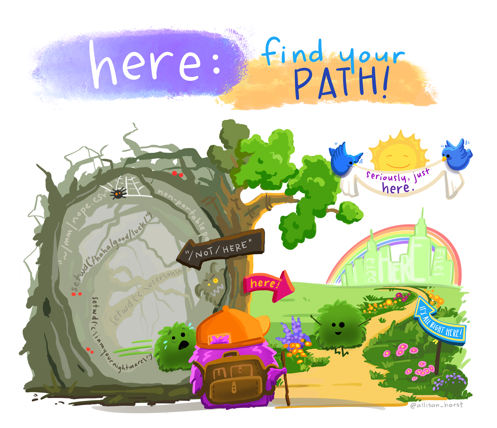
This means that as long as you are using an R project, and here::here your work is reproducible on anyone else’s computer also using an R project.

Extra path

Important

In my project for this website, these notes are stored in a notes folder, with a data subfolder. That’s why you will see the path as notes/data/. You will have to remove the notes portion of the path (everywhere) so that it works on your computer.

Advice: use CTRL+F to find notes/data and replace all with data.

Reading rectangular data into R

readr & readxl

read_csv() - comma delimited files
read_csv2() - semicolon separated files (common where , is the decimal place)
read_tsv() - tab delimited files
read_delim() - any delimiter
read_fwf() - fixed width files

read_excel() - read xls or xlsx files

Reading data

nobel <- read_csv(file = here::here("notes/data/nobel.csv"))
nobel

# A tibble: 935 × 26
      id firstname    surname  year category affiliation city  country
   <dbl> <chr>        <chr>   <dbl> <chr>    <chr>       <chr> <chr>  
 1     1 Wilhelm Con… Röntgen  1901 Physics  Munich Uni… Muni… Germany
 2     2 Hendrik A.   Lorentz  1902 Physics  Leiden Uni… Leid… Nether…
 3     3 Pieter       Zeeman   1902 Physics  Amsterdam … Amst… Nether…
 4     4 Henri        Becque…  1903 Physics  École Poly… Paris France 
 5     5 Pierre       Curie    1903 Physics  École muni… Paris France 
 6     6 Marie        Curie    1903 Physics  <NA>        <NA>  <NA>   
 7     6 Marie        Curie    1911 Chemist… Sorbonne U… Paris France 
 8     8 Lord         Raylei…  1904 Physics  Royal Inst… Lond… United…
 9     9 Philipp      Lenard   1905 Physics  Kiel Unive… Kiel  Germany
10    10 J.J.         Thomson  1906 Physics  University… Camb… United…
# ℹ 925 more rows
# ℹ 18 more variables: born_date <date>, died_date <date>,
#   gender <chr>, born_city <chr>, born_country <chr>,
#   born_country_code <chr>, died_city <chr>, died_country <chr>,
#   died_country_code <chr>, overall_motivation <chr>, share <dbl>,
#   motivation <chr>, born_country_original <chr>,
#   born_city_original <chr>, died_country_original <chr>, …

Writing data

Write a file

df <- tribble(
  ~x, ~y,
  1,  "a",
  2,  "b",
  3,  "c"
)

write_csv(df, file = here::here("notes/data/df.csv"))

Read it back in to inspect

read_csv(here::here("notes/data/df.csv"))

# A tibble: 3 × 2
      x y    
  <dbl> <chr>
1     1 a    
2     2 b    
3     3 c

Keep your raw data safe

One good practice to keep source data untouched is to put it in one folder (e.g. data-raw/) that you never overwrite, and write cleaned/derived files — like these two splits — to a separate data/ folder. That way you can always regenerate your cleaned data from the untouched original.

Variable names

Data with bad names

edibnb_badnames <- read_csv(here::here("notes/data/edibnb-badnames.csv"))
names(edibnb_badnames)

 [1] "ID"                   "Price"               
 [3] "neighbourhood"        "accommodates"        
 [5] "Number of bathrooms"  "Number of Bedrooms"  
 [7] "n beds"               "Review Scores Rating"
 [9] "Number of reviews"    "listing_url"

R doesn’t allow spaces in variable names:

ggplot(edibnb_badnames, aes(x = Number of bathrooms, y = Price)) +
  geom_point()

Error in parse(text = input): <text>:1:40: unexpected symbol
1: ggplot(edibnb_badnames, aes(x = Number of
                                           ^

Option 1 - Define column names

edibnb_col_names <- read_csv(here::here("notes/data/edibnb-badnames.csv"),
                             col_names = c("id", "price",
                                           "neighbourhood", "accommodates",
                                           "bathroom", "bedroom",
                                           "bed", "review_scores_rating",
                                           "n_reviews", "url"))

names(edibnb_col_names)

 [1] "id"                   "price"               
 [3] "neighbourhood"        "accommodates"        
 [5] "bathroom"             "bedroom"             
 [7] "bed"                  "review_scores_rating"
 [9] "n_reviews"            "url"

Option 2 - Format text to snake_case

edibnb_clean_names <- read_csv(here::here("notes/data/edibnb-badnames.csv")) %>%
  janitor::clean_names()

names(edibnb_clean_names)

 [1] "id"                   "price"               
 [3] "neighbourhood"        "accommodates"        
 [5] "number_of_bathrooms"  "number_of_bedrooms"  
 [7] "n_beds"               "review_scores_rating"
 [9] "number_of_reviews"    "listing_url"

Option 1. Explicit NAs

read_csv(here::here("notes/data/df-na.csv"),
         na = c("", "NA", ".", "9999", "Not applicable"))

# A tibble: 9 × 3
      x y     z     
  <dbl> <chr> <chr> 
1     1 a     hi    
2    NA b     hello 
3     3 <NA>  <NA>  
4     4 d     ola   
5     5 e     hola  
6    NA f     whatup
7     7 g     wassup
8     8 h     sup   
9     9 i     <NA>

Option 2. Specify column types

read_csv(here::here("notes/data/df-na.csv"), 
         col_types = list(col_double(), col_character(), col_character()))

# A tibble: 9 × 3
      x y              z     
  <dbl> <chr>          <chr> 
1     1 a              hi    
2    NA b              hello 
3     3 Not applicable 9999  
4     4 d              ola   
5     5 e              hola  
6    NA f              whatup
7     7 g              wassup
8     8 h              sup   
9     9 i              <NA>

Column types

type function	data type
`col_character()`	character
`col_date()`	date
`col_datetime()`	POSIXct (date-time)
`col_double()`	double (numeric)
`col_factor()`	factor
`col_guess()`	let readr guess (default)
`col_integer()`	integer
`col_logical()`	logical
`col_number()`	numbers mixed with non-number characters
`col_numeric()`	double or integer
`col_skip()`	do not read
`col_time()`	time

Where do these types come from?

read_csv(here::here("notes/data/df-na.csv"))

Rows: 9 Columns: 3
── Column specification ──────────────────────────────────────────────
Delimiter: ","
chr (3): x, y, z

ℹ Use `spec()` to retrieve the full column specification for this data.
ℹ Specify the column types or set `show_col_types = FALSE` to quiet this message.

# A tibble: 9 × 3
  x     y              z     
  <chr> <chr>          <chr> 
1 1     a              hi    
2 <NA>  b              hello 
3 3     Not applicable 9999  
4 4     d              ola   
5 5     e              hola  
6 .     f              whatup
7 7     g              wassup
8 8     h              sup   
9 9     i              <NA>

readr prints the column type guesses it made when parsing — that’s the same vocabulary as the table on the last slide.

Case study: Favorite foods

Read the data

fav_food <- read_excel(here::here("notes/data/favourite-food.xlsx"))

fav_food

# A tibble: 5 × 6
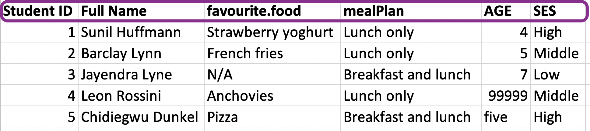
  `Student ID` `Full Name`      favourite.food    mealPlan AGE   SES  
         <dbl> <chr>            <chr>             <chr>    <chr> <chr>
1            1 Sunil Huffmann   Strawberry yoghu… Lunch o… 4     High 
2            2 Barclay Lynn     French fries      Lunch o… 5     Midd…
3            3 Jayendra Lyne    N/A               Breakfa… 7     Low  
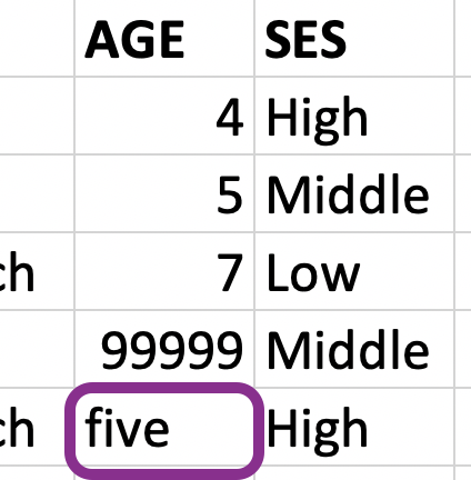
4            4 Leon Rossini     Anchovies         Lunch o… 99999 Midd…
5            5 Chidiegwu Dunkel Pizza             Breakfa… five  High

Clean the names

fav_food <- read_excel(here::here("notes/data/favourite-food.xlsx")) %>%
  janitor::clean_names()

fav_food

# A tibble: 5 × 6
  student_id full_name        favourite_food     meal_plan age   ses  
       <dbl> <chr>            <chr>              <chr>     <chr> <chr>
1          1 Sunil Huffmann   Strawberry yoghurt Lunch on… 4     High 
2          2 Barclay Lynn     French fries       Lunch on… 5     Midd…
3          3 Jayendra Lyne    N/A                Breakfas… 7     Low  
4          4 Leon Rossini     Anchovies          Lunch on… 99999 Midd…
5          5 Chidiegwu Dunkel Pizza              Breakfas… five  High

Handle NAs

fav_food <- read_excel(here::here("notes/data/favourite-food.xlsx"),
                       na = c("N/A", "99999")) %>%
  janitor::clean_names()

fav_food

# A tibble: 5 × 6
  student_id full_name        favourite_food     meal_plan age   ses  
       <dbl> <chr>            <chr>              <chr>     <chr> <chr>
1          1 Sunil Huffmann   Strawberry yoghurt Lunch on… 4     High 
2          2 Barclay Lynn     French fries       Lunch on… 5     Midd…
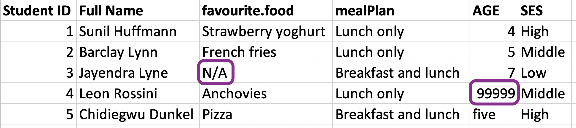
3          3 Jayendra Lyne    <NA>               Breakfas… 7     Low  
4          4 Leon Rossini     Anchovies          Lunch on… <NA>  Midd…
5          5 Chidiegwu Dunkel Pizza              Breakfas… five  High

Make `age` numeric

fav_food <- fav_food %>%
  mutate(
    age = if_else(age == "five", "5", age),
    age = as.numeric(age)
    )

glimpse(fav_food)

Rows: 5
Columns: 6
$ student_id     <dbl> 1, 2, 3, 4, 5
$ full_name      <chr> "Sunil Huffmann", "Barclay Lynn", "Jayendra L…
$ favourite_food <chr> "Strawberry yoghurt", "French fries", NA, "An…
$ meal_plan      <chr> "Lunch only", "Lunch only", "Breakfast and lu…
$ age            <dbl> 4, 5, 7, NA, 5
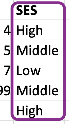
$ ses            <chr> "High", "Middle", "Low", "Middle", "High"

Socio-economic status

What order are the levels of ses listed in?

fav_food %>%
  count(ses)

# A tibble: 3 × 2
  ses        n
  <chr>  <int>
1 High       2
2 Low        1
3 Middle     2

Make `ses` a factor

fav_food <- fav_food %>%
  mutate(ses = fct_relevel(ses, "Low", "Middle", "High"))

fav_food %>%
  count(ses)

# A tibble: 3 × 2
  ses        n
  <fct>  <int>
1 Low        1
2 Middle     2
3 High       2

Putting it all together

fav_food <- read_excel(here::here("notes/data/favourite-food.xlsx"), 
                       na = c("N/A", "99999")) %>%
  janitor::clean_names() %>%
  mutate(
    age = if_else(age == "five", "5", age),
    age = as.numeric(age),
    ses = fct_relevel(ses, "Low", "Middle", "High")
  )

fav_food

# A tibble: 5 × 6
  student_id full_name        favourite_food     meal_plan   age ses  
       <dbl> <chr>            <chr>              <chr>     <dbl> <fct>
1          1 Sunil Huffmann   Strawberry yoghurt Lunch on…     4 High 
2          2 Barclay Lynn     French fries       Lunch on…     5 Midd…
3          3 Jayendra Lyne    <NA>               Breakfas…     7 Low  
4          4 Leon Rossini     Anchovies          Lunch on…    NA Midd…
5          5 Chidiegwu Dunkel Pizza              Breakfas…     5 High

Out and back in

write_csv(fav_food, file = here::here("notes/data/fav-food-clean.csv"))

fav_food_clean <- read_csv(here::here("notes/data/fav-food-clean.csv"))

What happened to ses again?

fav_food_clean %>%
  count(ses)

# A tibble: 3 × 2
  ses        n
  <chr>  <int>
1 High       2
2 Low        1
3 Middle     2

CSVs don’t store variable type information, so ses comes back as plain character — the factor ordering is lost.

`read_rds()` and `write_rds()`

CSVs can be unreliable for saving interim results if there is specific variable type information you want to keep.
RDS files preserve it — read and write them with read_rds() and write_rds().

read_rds(path)
write_rds(x, path)

Out and back in, take 2

write_rds(fav_food, file = here::here("notes/data/fav-food-clean.rds"))

fav_food_clean <- read_rds(here::here("notes/data/fav-food-clean.rds"))

fav_food_clean %>%
  count(ses)

# A tibble: 3 × 2
  ses        n
  <fct>  <int>
1 Low        1
2 Middle     2
3 High       2

This time ses keeps its factor levels and order.

Other types of data

googlesheets4: Google Sheets
haven: SPSS, Stata, and SAS files
DBI, plus a database-specific backend (e.g. RMySQL, RSQLite, RPostgreSQL): run SQL queries against a database and return a data frame
jsonlite: JSON
xml2: XML
rvest: web scraping
httr: web APIs
sparklyr: data loaded into Spark

Acknowledgements & Credits

Note

This page adapts material from Data Science in a Box (Unit 2, Deck 12: “Importing data”) by Mine Çetinkaya-Rundel, licensed under CC BY-SA 4.0. Source: tidyverse/datascience-box. Modified: converted from xaringan to Quarto revealjs; added content on here::here()

Importing Data

Setup

Dr. D’s note on file paths

Extra path

Reading rectangular data into R

readr & readxl

Reading data

Writing data

Keep your raw data safe

Variable names

Data with bad names

Option 1 - Define column names

Option 2 - Format text to snake_case

Option 1. Explicit NAs

Option 2. Specify column types

Column types

Where do these types come from?

Case study: Favorite foods

Read the data

Clean the names

Handle NAs

Make age numeric

Socio-economic status

Make ses a factor

Putting it all together

Out and back in

read_rds() and write_rds()

Out and back in, take 2

Other types of data

Other types of data

Acknowledgements & Credits

Make `age` numeric

Make `ses` a factor

`read_rds()` and `write_rds()`