Data classes

wk5-d02-data-classes

Dr. D

Chico State
DATA 385 - Fall 2026

September 23, 2026

Setup

🎥 Data classes - code along in wk5-d02

library(tidyverse)
library(glue) # new! Install it before first use. 

New Packages

glue: glue() makes it easy to interpolate data into strings:

Data classes

Data classes

We talked about types so far, next we’ll introduce the concept of classes.

  • Vectors are like Lego building blocks
  • We stick them together to build more complicated constructs, e.g. representations of data
  • The class attribute relates to the S3 class of an object, which determines its behavior
  • Examples: factors, dates, and data frames

Factors

R uses factors to handle categorical variables — variables that have a fixed and known set of possible values.

x <- factor(c("BS", "MS", "PhD", "MS"))
x
[1] BS  MS  PhD MS 
Levels: BS MS PhD
typeof(x)
[1] "integer"
class(x)
[1] "factor"

More on factors

We can think of factors as character (level labels) and integer (level numbers) glued together.

glimpse(x)
 Factor w/ 3 levels "BS","MS","PhD": 1 2 3 2
as.integer(x)
[1] 1 2 3 2

Dates

y <- as.Date("2020-01-01")
y
[1] "2020-01-01"
typeof(y)
[1] "double"
class(y)
[1] "Date"

More on dates

We can think of dates as an integer (the number of days since the origin, 1 Jan 1970) glued together with that origin.

as.integer(y)
[1] 18262
as.integer(y) / 365 # roughly 50 yrs
[1] 50.03288

Data frames

We can think of data frames as vectors of equal length glued together.

df <- data.frame(x = 1:2, y = 3:4)
df
  x y
1 1 3
2 2 4
typeof(df)
[1] "list"
class(df)
[1] "data.frame"

Lists

Lists are a generic vector container — vectors of any type can go in them.

l <- list(
  x = 1:4,
  y = c("hi", "hello", "jello"),
  z = c(TRUE, FALSE)
)
l
$x
[1] 1 2 3 4

$y
[1] "hi"    "hello" "jello"

$z
[1]  TRUE FALSE

Lists and data frames

  • A data frame is a special list containing vectors of equal length
  • When we use the pull() function, we extract a vector from the data frame
df
  x y
1 1 3
2 2 4
df %>%
  pull(y)
[1] 3 4

Working with factors

Read data in as character strings

glimpse(cat_lovers)
Rows: 60
Columns: 3
$ name           <chr> "Bernice Warren", "Woodrow Stone", "Willie Ba…
$ number_of_cats <chr> "0", "0", "1", "3", "3", "2", "1", "1", "0", …
$ handedness     <chr> "left", "left", "left", "left", "left", "left…

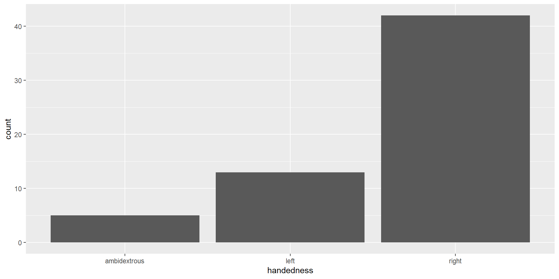
But coerce when plotting

ggplot(cat_lovers, mapping = aes(x = handedness)) +
  geom_bar()

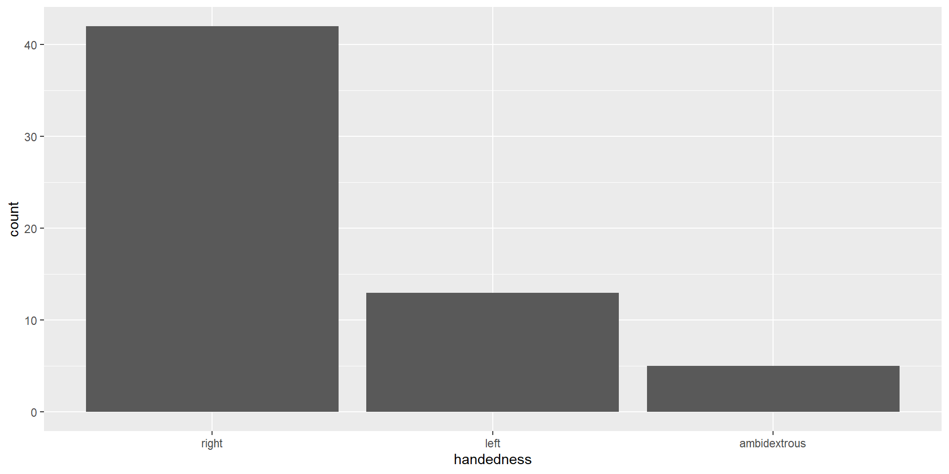
Use forcats to manipulate factors

cat_lovers %>%
  mutate(handedness = fct_infreq(handedness)) %>%
  ggplot(mapping = aes(x = handedness)) +
  geom_bar()

Come for the functionality…

… stay for the logo

  • Factors are useful when you have true categorical data and you want to override the ordering of character vectors to improve display
  • They are also useful in modeling scenarios
  • The forcats package provides a suite of useful tools that solve common problems with factors

Working with dates

Make a date

  • lubridate is the tidyverse-friendly package that makes dealing with dates a little easier
  • It’s not one of the core tidyverse packages — it’s installed with install.packages("tidyverse") but not loaded with it, so it needs to be explicitly loaded with
library(lubridate)

Goal: Calculate and visualize the number of bookings on any given arrival date.

hotels <- read_csv("data/hotels.csv")
hotels %>% select(starts_with("arrival_"))
# A tibble: 119,390 × 4
   arrival_date_year arrival_date_month arrival_date_week_number
               <dbl> <chr>                                 <dbl>
 1              2015 July                                     27
 2              2015 July                                     27
 3              2015 July                                     27
 4              2015 July                                     27
 5              2015 July                                     27
 6              2015 July                                     27
 7              2015 July                                     27
 8              2015 July                                     27
 9              2015 July                                     27
10              2015 July                                     27
# ℹ 119,380 more rows
# ℹ 1 more variable: arrival_date_day_of_month <dbl>

Step 1. Construct dates

hotels %>%
  mutate(
    arrival_date = glue("{arrival_date_year} {arrival_date_month} {arrival_date_day_of_month}")
    ) %>%
  relocate(arrival_date) # move this variable to the front of the line!
# A tibble: 119,390 × 33
   arrival_date hotel        is_canceled lead_time arrival_date_year
   <glue>       <chr>              <dbl>     <dbl>             <dbl>
 1 2015 July 1  Resort Hotel           0       342              2015
 2 2015 July 1  Resort Hotel           0       737              2015
 3 2015 July 1  Resort Hotel           0         7              2015
 4 2015 July 1  Resort Hotel           0        13              2015
 5 2015 July 1  Resort Hotel           0        14              2015
 6 2015 July 1  Resort Hotel           0        14              2015
 7 2015 July 1  Resort Hotel           0         0              2015
 8 2015 July 1  Resort Hotel           0         9              2015
 9 2015 July 1  Resort Hotel           1        85              2015
10 2015 July 1  Resort Hotel           1        75              2015
# ℹ 119,380 more rows
# ℹ 28 more variables: arrival_date_month <chr>,
#   arrival_date_week_number <dbl>, arrival_date_day_of_month <dbl>,
#   stays_in_weekend_nights <dbl>, stays_in_week_nights <dbl>,
#   adults <dbl>, children <dbl>, babies <dbl>, meal <chr>,
#   country <chr>, market_segment <chr>, distribution_channel <chr>,
#   is_repeated_guest <dbl>, previous_cancellations <dbl>, …

Step 2. Count bookings per date

hotels %>%
  mutate(arrival_date = glue("{arrival_date_year} {arrival_date_month} {arrival_date_day_of_month}")) %>%
  count(arrival_date)
# A tibble: 793 × 2
   arrival_date       n
   <glue>         <int>
 1 2015 August 1    110
 2 2015 August 10   207
 3 2015 August 11   117
 4 2015 August 12   133
 5 2015 August 13   107
 6 2015 August 14   329
 7 2015 August 15   190
 8 2015 August 16    98
 9 2015 August 17   188
10 2015 August 18    94
# ℹ 783 more rows

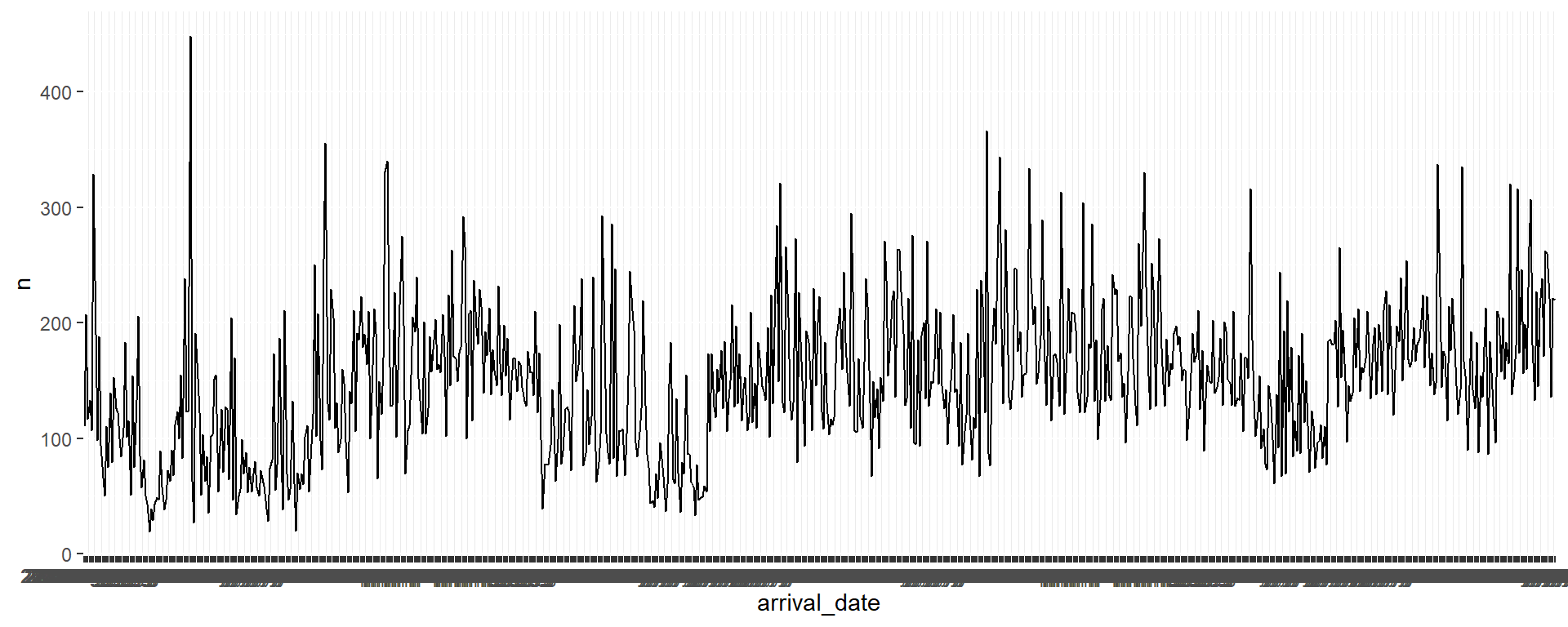
Step 3. Visualize bookings per date

hotels %>%
  mutate(arrival_date = glue("{arrival_date_year} {arrival_date_month} {arrival_date_day_of_month}")) %>%
  count(arrival_date) %>%
  ggplot(aes(x = arrival_date, y = n, group = 1)) +
  geom_line()

Zooming in a bit…

Why does the plot start with August when we know our data start in July? And why does 10 August come after 1 August?
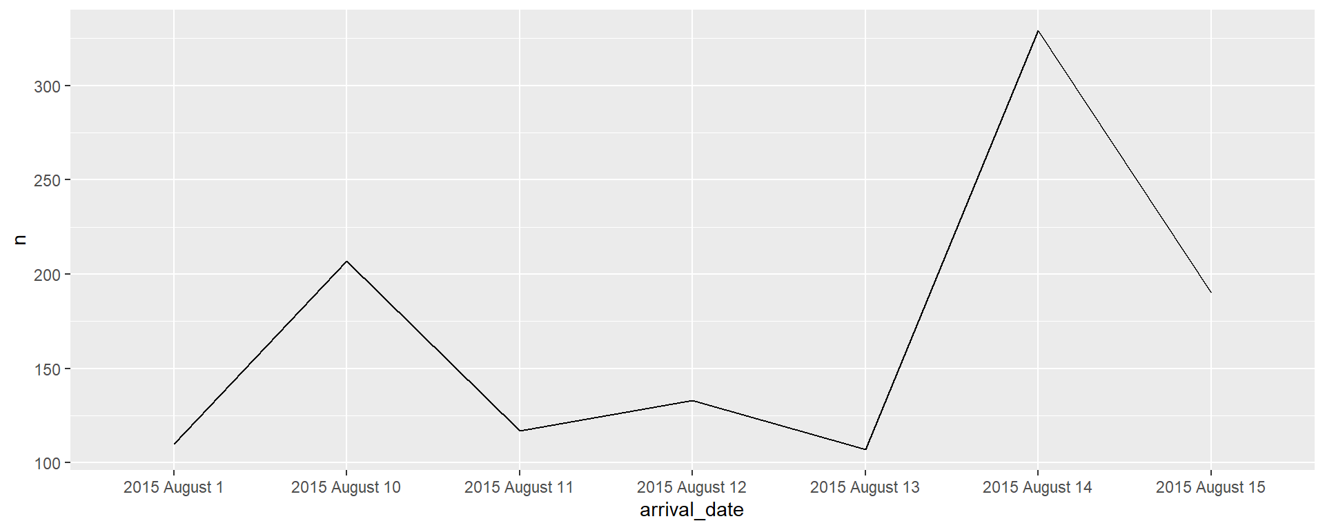
Code
hotels %>%
  mutate(arrival_date = glue("{arrival_date_year} {arrival_date_month} {arrival_date_day_of_month}")) %>%
  count(arrival_date) %>%
  slice(1:7) %>%
  ggplot(aes(x = arrival_date, y = n, group = 1)) +
  geom_line()

The dates are still character strings — they sort alphabetically, not chronologically.

Step 1, revised. Construct dates as dates

hotels %>%
  mutate(
    arrival_date = ymd(glue("{arrival_date_year} {arrival_date_month} {arrival_date_day_of_month}"))
    ) %>%
  relocate(arrival_date)
# A tibble: 119,390 × 33
   arrival_date hotel        is_canceled lead_time arrival_date_year
   <date>       <chr>              <dbl>     <dbl>             <dbl>
 1 2015-07-01   Resort Hotel           0       342              2015
 2 2015-07-01   Resort Hotel           0       737              2015
 3 2015-07-01   Resort Hotel           0         7              2015
 4 2015-07-01   Resort Hotel           0        13              2015
 5 2015-07-01   Resort Hotel           0        14              2015
 6 2015-07-01   Resort Hotel           0        14              2015
 7 2015-07-01   Resort Hotel           0         0              2015
 8 2015-07-01   Resort Hotel           0         9              2015
 9 2015-07-01   Resort Hotel           1        85              2015
10 2015-07-01   Resort Hotel           1        75              2015
# ℹ 119,380 more rows
# ℹ 28 more variables: arrival_date_month <chr>,
#   arrival_date_week_number <dbl>, arrival_date_day_of_month <dbl>,
#   stays_in_weekend_nights <dbl>, stays_in_week_nights <dbl>,
#   adults <dbl>, children <dbl>, babies <dbl>, meal <chr>,
#   country <chr>, market_segment <chr>, distribution_channel <chr>,
#   is_repeated_guest <dbl>, previous_cancellations <dbl>, …

ymd() is the function from lubridate package that is used here.

Step 2. Count bookings per date

hotels %>%
  mutate(arrival_date = ymd(glue("{arrival_date_year} {arrival_date_month} {arrival_date_day_of_month}"))) %>%
  count(arrival_date)
# A tibble: 793 × 2
   arrival_date     n
   <date>       <int>
 1 2015-07-01     122
 2 2015-07-02      93
 3 2015-07-03      56
 4 2015-07-04      88
 5 2015-07-05      53
 6 2015-07-06      75
 7 2015-07-07      54
 8 2015-07-08      69
 9 2015-07-09      80
10 2015-07-10      51
# ℹ 783 more rows

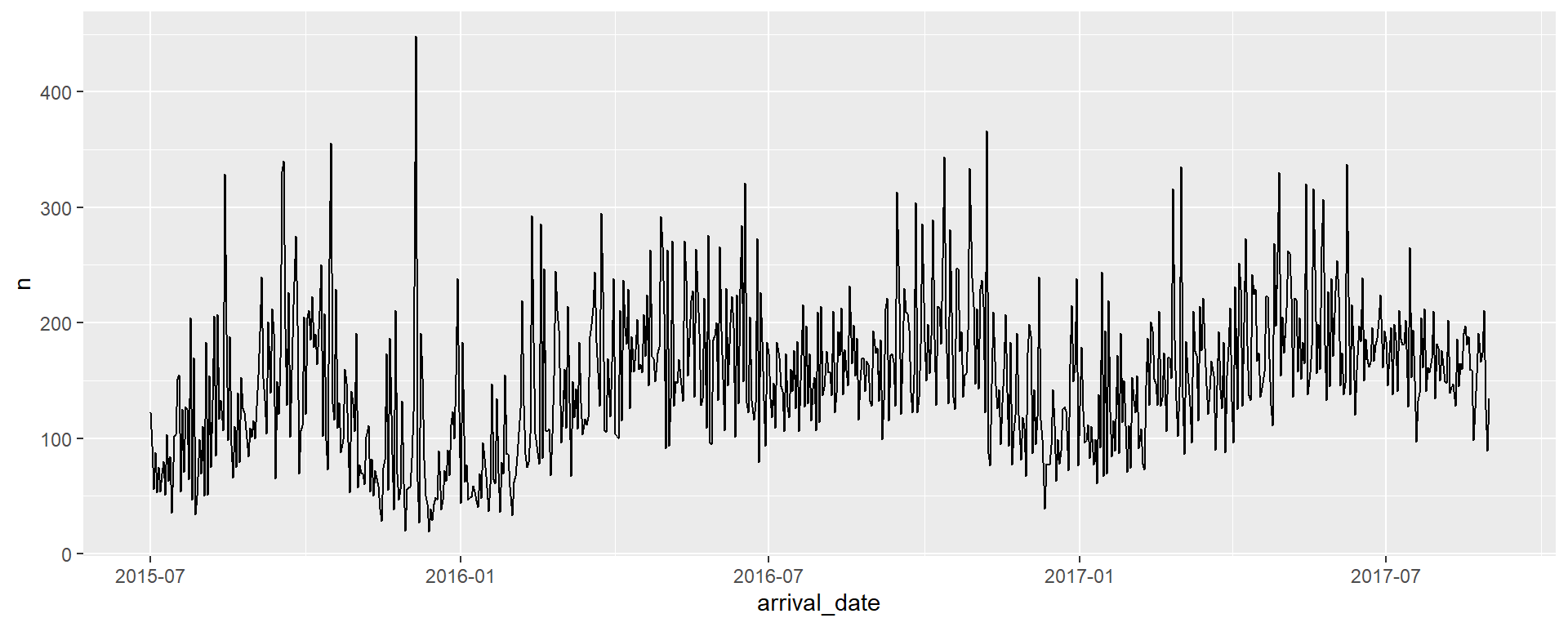
Step 3a. Visualize bookings per date

hotels %>%
  mutate(arrival_date = ymd(glue("{arrival_date_year} {arrival_date_month} {arrival_date_day_of_month}"))) %>%
  count(arrival_date) %>%
  ggplot(aes(x = arrival_date, y = n, group = 1)) +
  geom_line()

Step 3b. Visualize using a smooth curve
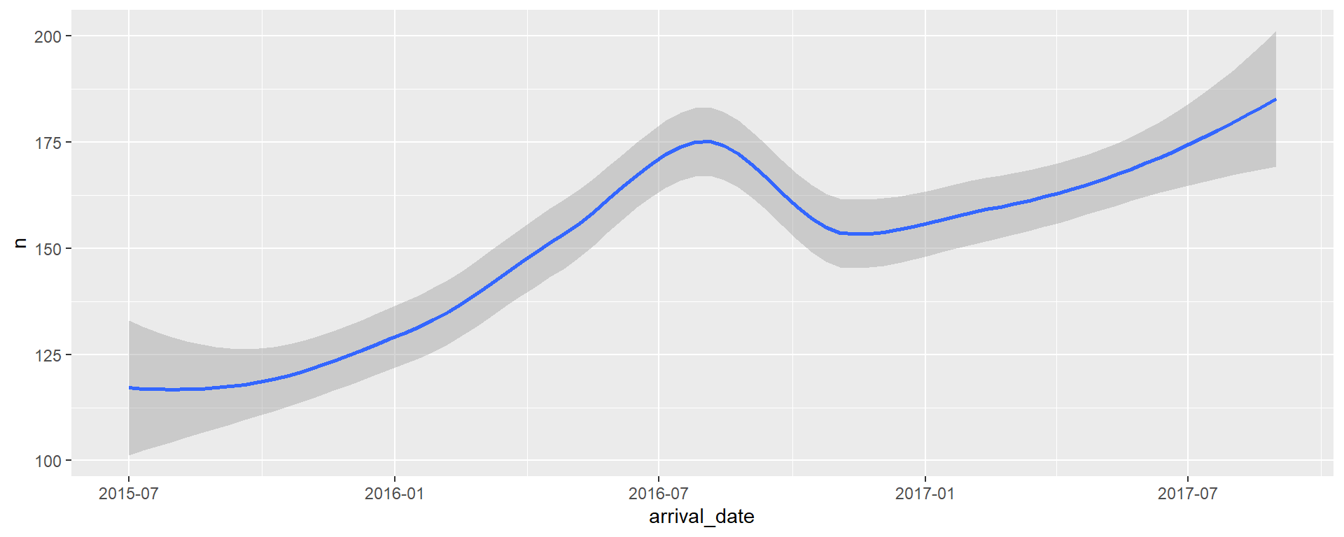
hotels %>%
  mutate(arrival_date = ymd(glue("{arrival_date_year} {arrival_date_month} {arrival_date_day_of_month}"))) %>%
  count(arrival_date) %>%
  ggplot(aes(x = arrival_date, y = n, group = 1)) +
  geom_smooth()

Acknowledgements & Credits

Note

This page adapts material from Data Science in a Box (Unit 2, Deck 11: “Data classes”) by Mine Çetinkaya-Rundel, licensed under CC BY-SA 4.0. Source: tidyverse/datascience-box. Modified: converted from xaringan to Quarto revealjs; reads hotels.csv from a local file instead of downloading it.