Visualising numerical data

wk2-d03-viz-num

Dr. D

Chico State
DATA 385 - Fall 2026

September 3, 2026

Get started

Setup

🎥 Numerical viz (24 min) - code along in wk2-d03

library(tidyverse)
library(openintro)
loans_full_schema <- loans_full_schema %>%
  mutate(grade = factor(grade, ordered = TRUE))

Terminology

Number of variables involved

Univariate data analysis - distribution of single variable
Bivariate data analysis - relationship between two variables
Multivariate data analysis - relationship between many variables at once, usually focusing on the relationship between two while conditioning for others

Types of variables

Numerical variables can be classified as continuous or discrete based on whether or not the variable can take on an infinite number of values or only non-negative whole numbers, respectively.
If the variable is categorical, we can determine if it is ordinal based on whether or not the levels have a natural ordering.

Data

Data: Lending Club

Thousands of loans made through the Lending Club, which is a platform that allows individuals to lend to other individuals
Not all loans are created equal – ease of getting a loan depends on (apparent) ability to pay back the loan
Data includes loans made, these are not loan applications

Take a peek at data

library(openintro)
glimpse(loans_full_schema)

Rows: 10,000
Columns: 55
$ emp_title                        <chr> "global config engineer ", …
$ emp_length                       <dbl> 3, 10, 3, 1, 10, NA, 10, 10…
$ state                            <fct> NJ, HI, WI, PA, CA, KY, MI,…
$ homeownership                    <fct> MORTGAGE, RENT, RENT, RENT,…
$ annual_income                    <dbl> 90000, 40000, 40000, 30000,…
$ verified_income                  <fct> Verified, Not Verified, Sou…
$ debt_to_income                   <dbl> 18.01, 5.04, 21.15, 10.16, …
$ annual_income_joint              <dbl> NA, NA, NA, NA, 57000, NA, …
$ verification_income_joint        <fct> , , , , Verified, , Not Ver…
$ debt_to_income_joint             <dbl> NA, NA, NA, NA, 37.66, NA, …
$ delinq_2y                        <int> 0, 0, 0, 0, 0, 1, 0, 1, 1, …
$ months_since_last_delinq         <int> 38, NA, 28, NA, NA, 3, NA, …
$ earliest_credit_line             <dbl> 2001, 1996, 2006, 2007, 200…
$ inquiries_last_12m               <int> 6, 1, 4, 0, 7, 6, 1, 1, 3, …
$ total_credit_lines               <int> 28, 30, 31, 4, 22, 32, 12, …
$ open_credit_lines                <int> 10, 14, 10, 4, 16, 12, 10, …
$ total_credit_limit               <int> 70795, 28800, 24193, 25400,…
$ total_credit_utilized            <int> 38767, 4321, 16000, 4997, 5…
$ num_collections_last_12m         <int> 0, 0, 0, 0, 0, 0, 0, 0, 0, …
$ num_historical_failed_to_pay     <int> 0, 1, 0, 1, 0, 0, 0, 0, 0, …
$ months_since_90d_late            <int> 38, NA, 28, NA, NA, 60, NA,…
$ current_accounts_delinq          <int> 0, 0, 0, 0, 0, 0, 0, 0, 0, …
$ total_collection_amount_ever     <int> 1250, 0, 432, 0, 0, 0, 0, 0…
$ current_installment_accounts     <int> 2, 0, 1, 1, 1, 0, 2, 2, 6, …
$ accounts_opened_24m              <int> 5, 11, 13, 1, 6, 2, 1, 4, 1…
$ months_since_last_credit_inquiry <int> 5, 8, 7, 15, 4, 5, 9, 7, 4,…
$ num_satisfactory_accounts        <int> 10, 14, 10, 4, 16, 12, 10, …
$ num_accounts_120d_past_due       <int> 0, 0, 0, 0, 0, 0, 0, NA, 0,…
$ num_accounts_30d_past_due        <int> 0, 0, 0, 0, 0, 0, 0, 0, 0, …
$ num_active_debit_accounts        <int> 2, 3, 3, 2, 10, 1, 3, 5, 11…
$ total_debit_limit                <int> 11100, 16500, 4300, 19400, …
$ num_total_cc_accounts            <int> 14, 24, 14, 3, 20, 27, 8, 1…
$ num_open_cc_accounts             <int> 8, 14, 8, 3, 15, 12, 7, 12,…
$ num_cc_carrying_balance          <int> 6, 4, 6, 2, 13, 5, 6, 10, 1…
$ num_mort_accounts                <int> 1, 0, 0, 0, 0, 3, 2, 7, 2, …
$ account_never_delinq_percent     <dbl> 92.9, 100.0, 93.5, 100.0, 1…
$ tax_liens                        <int> 0, 0, 0, 1, 0, 0, 0, 0, 0, …
$ public_record_bankrupt           <int> 0, 1, 0, 0, 0, 0, 0, 0, 0, …
$ loan_purpose                     <fct> moving, debt_consolidation,…
$ application_type                 <fct> individual, individual, ind…
$ loan_amount                      <int> 28000, 5000, 2000, 21600, 2…
$ term                             <dbl> 60, 36, 36, 36, 36, 36, 60,…
$ interest_rate                    <dbl> 14.07, 12.61, 17.09, 6.72, …
$ installment                      <dbl> 652.53, 167.54, 71.40, 664.…
$ grade                            <ord> C, C, D, A, C, A, C, B, C, …
$ sub_grade                        <fct> C3, C1, D1, A3, C3, A3, C2,…
$ issue_month                      <fct> Mar-2018, Feb-2018, Feb-201…
$ loan_status                      <fct> Current, Current, Current, …
$ initial_listing_status           <fct> whole, whole, fractional, w…
$ disbursement_method              <fct> Cash, Cash, Cash, Cash, Cas…
$ balance                          <dbl> 27015.86, 4651.37, 1824.63,…
$ paid_total                       <dbl> 1999.330, 499.120, 281.800,…
$ paid_principal                   <dbl> 984.14, 348.63, 175.37, 274…
$ paid_interest                    <dbl> 1015.19, 150.49, 106.43, 56…
$ paid_late_fees                   <dbl> 0, 0, 0, 0, 0, 0, 0, 0, 0, …

note that this has 55 columns

Selected variables

today we are only going to look at the following variables. take full data, pipe that into select to only choose some vars, save it as new data

loans <- loans_full_schema %>%
  select(loan_amount, interest_rate, term, grade,
         state, annual_income, homeownership, debt_to_income)
glimpse(loans)

Rows: 10,000
Columns: 8
$ loan_amount    <int> 28000, 5000, 2000, 21600, 23000, 5000, 24000,…
$ interest_rate  <dbl> 14.07, 12.61, 17.09, 6.72, 14.07, 6.72, 13.59…
$ term           <dbl> 60, 36, 36, 36, 36, 36, 60, 60, 36, 36, 60, 6…
$ grade          <ord> C, C, D, A, C, A, C, B, C, A, C, B, C, B, D, …
$ state          <fct> NJ, HI, WI, PA, CA, KY, MI, AZ, NV, IL, IL, F…
$ annual_income  <dbl> 90000, 40000, 40000, 30000, 35000, 34000, 350…
$ homeownership  <fct> MORTGAGE, RENT, RENT, RENT, RENT, OWN, MORTGA…
$ debt_to_income <dbl> 18.01, 5.04, 21.15, 10.16, 57.96, 6.46, 23.66…

loan_amount: Amount of the loan received, in US dollars
interest_rate: Interest rate on the loan, in an annual percentage
term: The length of the loan, which is always set as a whole number of months
grade: Loan grade, which takes a values A through G and represents the quality of the loan and its likelihood of being repaid
state: US state where the borrower resides
annual_income: Borrower’s annual income, including any second income, in US dollars
homeownership: Indicates whether the person owns, owns but has a mortgage, or rents
debt_to_income: Debt-to-income ratio

Variable types

loan_amount: numerical, continuous
interest_rate: numerical, continuous
term: numerical, discrete
grade: categorical, ordinal
state: categorical, not ordinal
annual_income: numerical, continuous
homeownership: categorical, not ordinal
debt_to_income: numerical, continuous

Visualizing numerical data

Describing shapes of numerical distributions

shape:
- skewness: right-skewed, left-skewed, symmetric (skew is to the side of the longer tail)
- modality: unimodal, bimodal, multimodal, uniform
center: mean (mean), median (median), mode (not always useful)
spread: range (range), standard deviation (sd), inter-quartile range (IQR)
unusual observations

Histogram

explain how to read the histogram (x and y axis, height of bars)

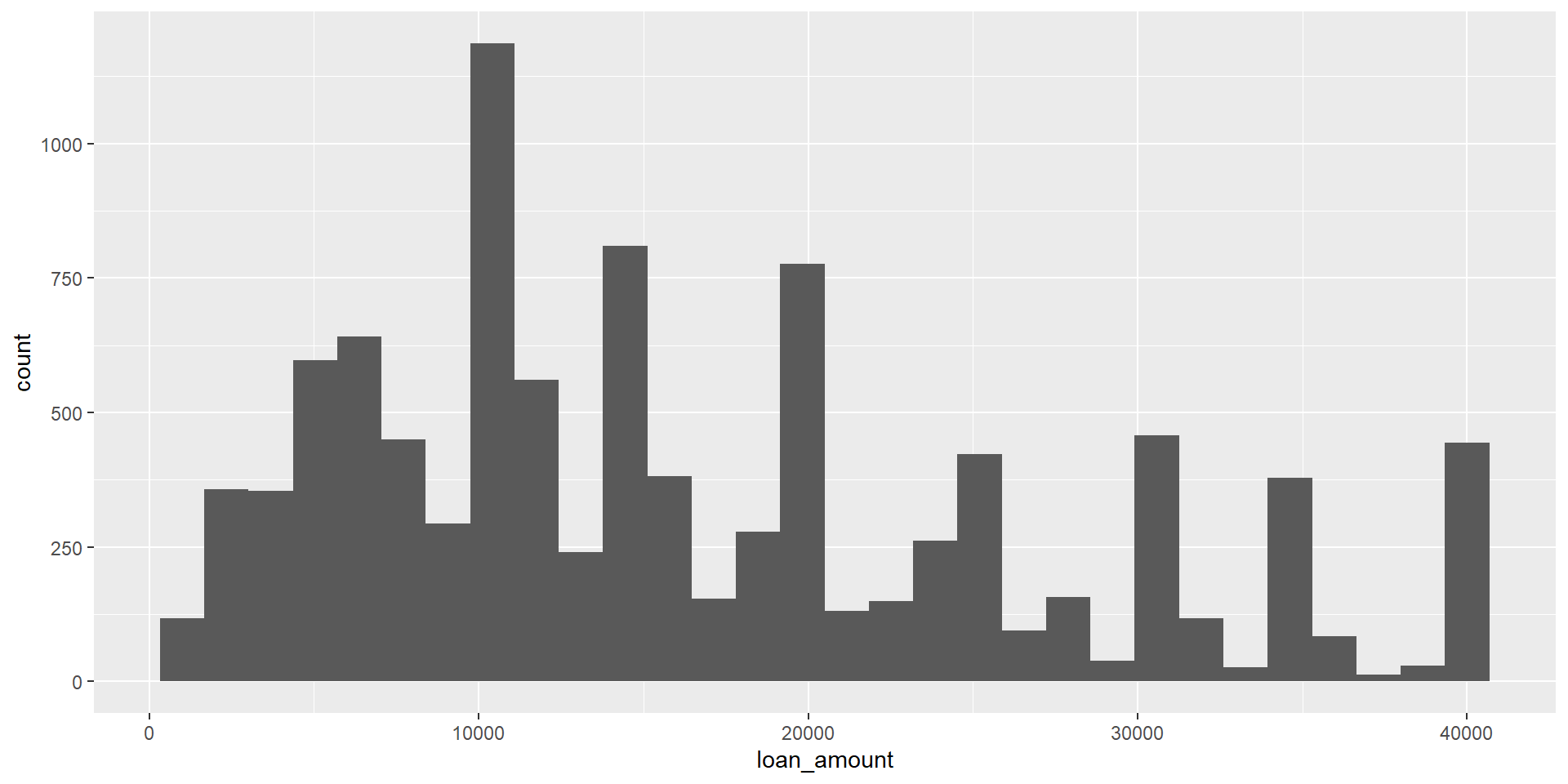
ggplot(loans, aes(x = loan_amount)) +
  geom_histogram()

explain the message about binwidth

Histograms and binwidth

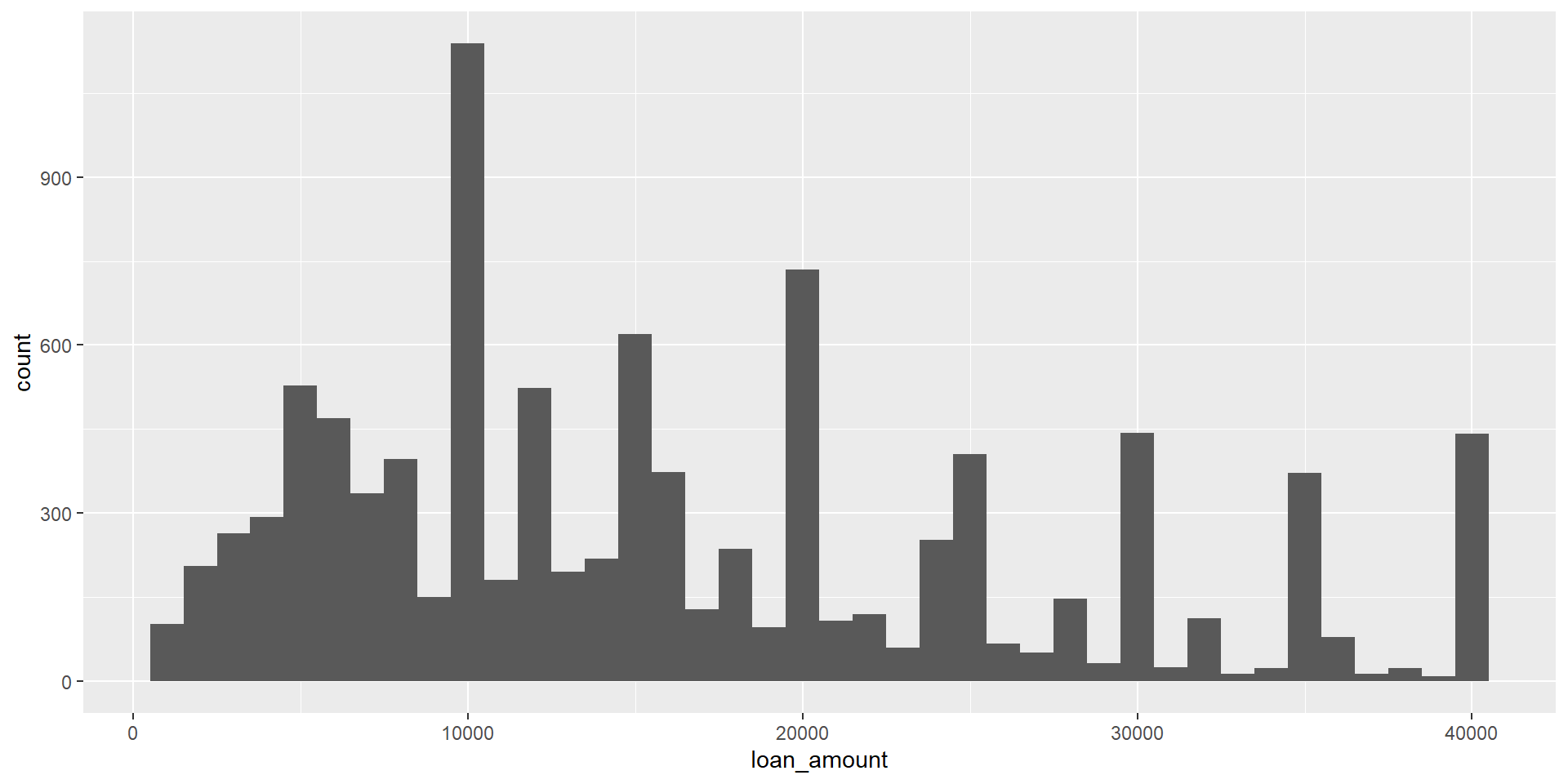
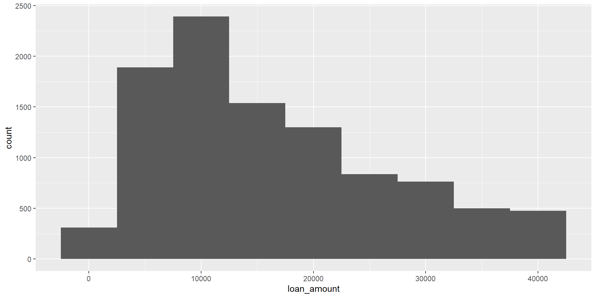
ggplot(loans, aes(x = loan_amount)) + geom_histogram(binwidth = 1000)
ggplot(loans, aes(x = loan_amount)) + geom_histogram(binwidth = 5000)
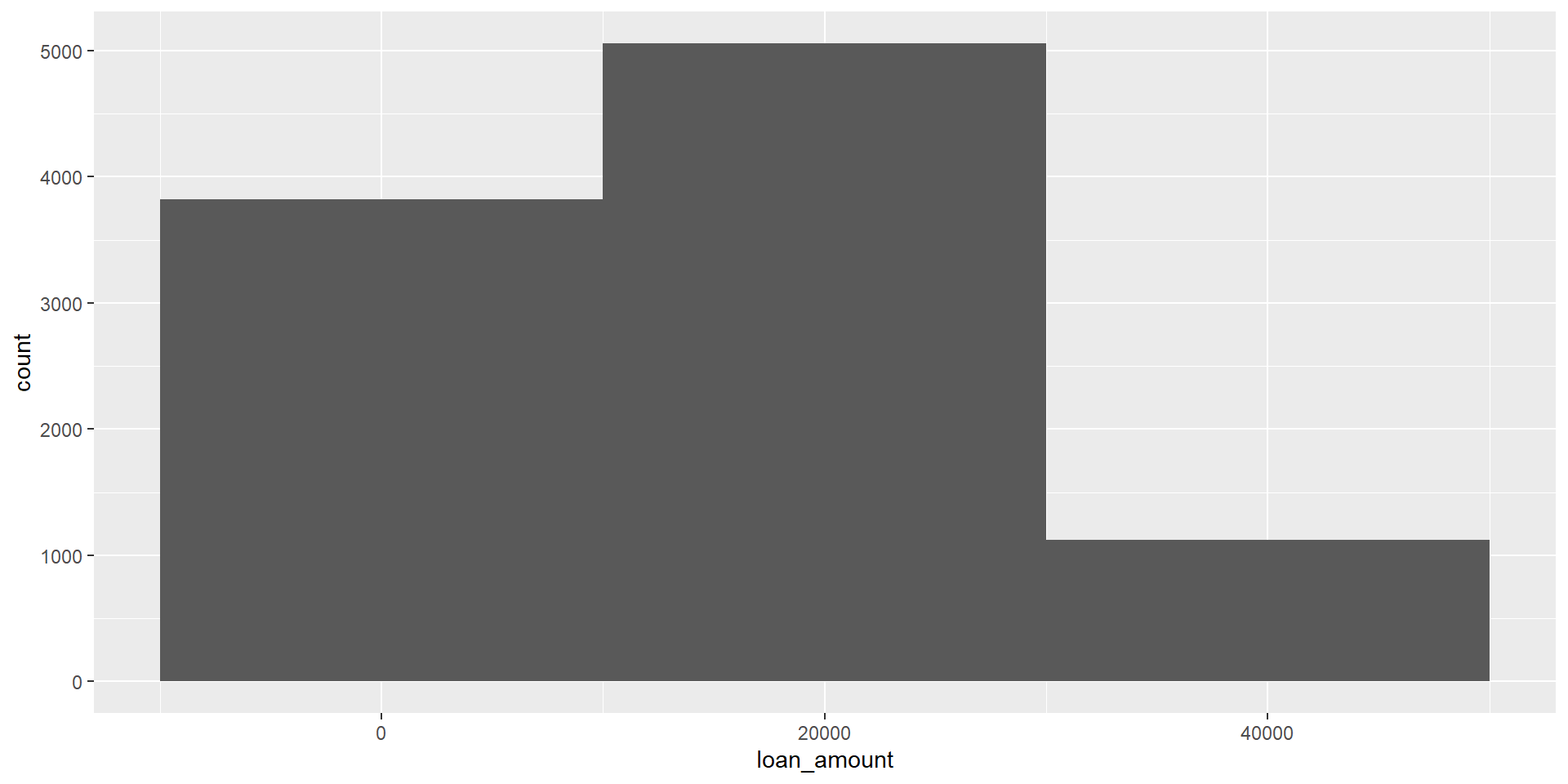
ggplot(loans, aes(x = loan_amount)) + geom_histogram(binwidth = 20000)

Modifying the binwidth can help you understand the shape of the distribution and can be influenced by the units of the variable (e.g. binwidth of 1 doesn’t make sense). balance between too jagged and too coarse.

Customizing histograms

gave axis labels and title

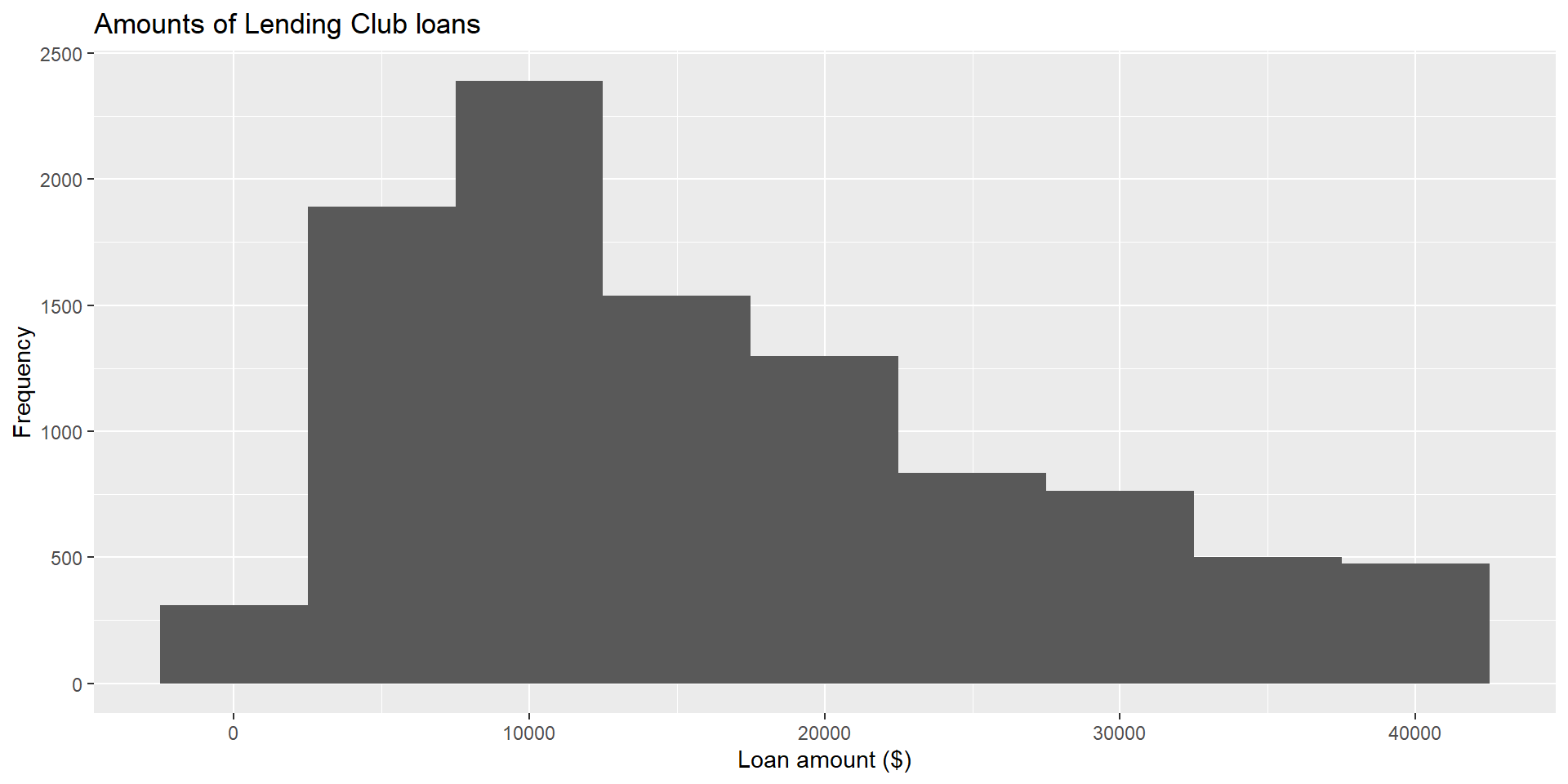
ggplot(loans, aes(x = loan_amount)) +
  geom_histogram(binwidth = 5000) +
  labs(
    x = "Loan amount ($)",
    y = "Frequency",
    title = "Amounts of Lending Club loans"
  )

Fill with a categorical variable

allows us to explore relationships between numeric and categorical variables add a new aestetic for fill, and alpha

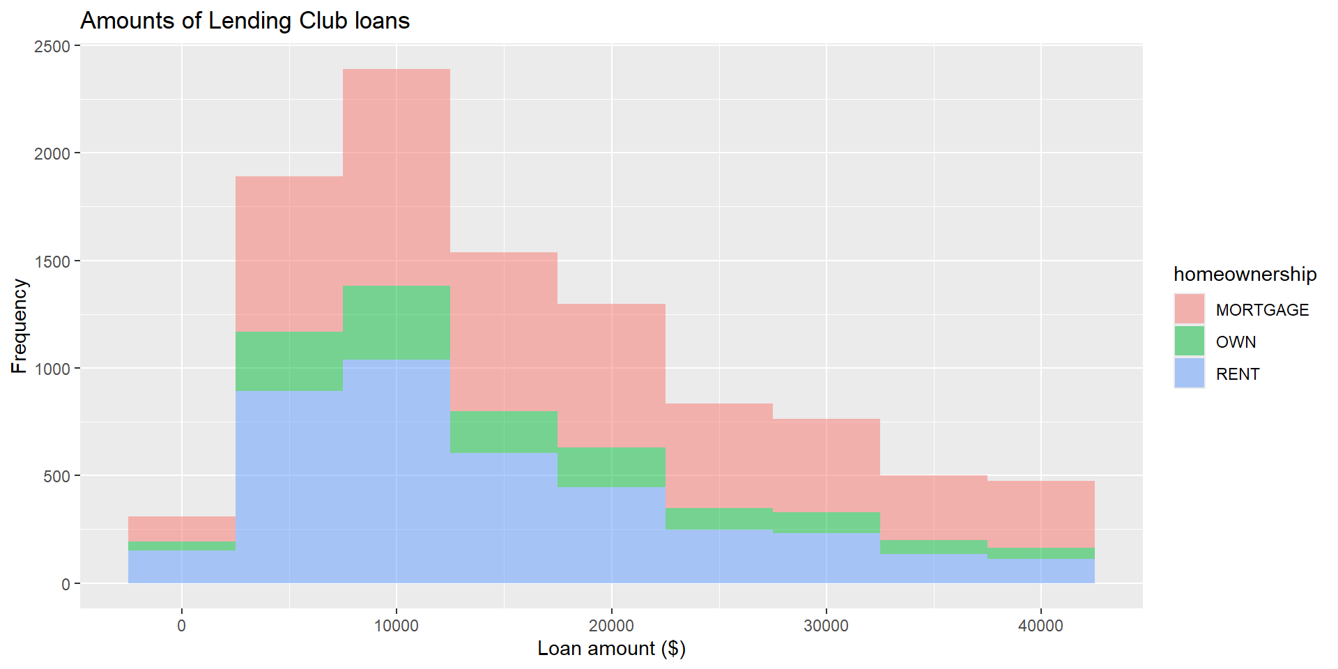
ggplot(loans, aes(x = loan_amount,
                  fill = homeownership)) +
  geom_histogram(binwidth = 5000,alpha = 0.5) +
  labs(
    x = "Loan amount ($)",
    y = "Frequency",
    title = "Amounts of Lending Club loans"
  )

but hard to tell if this is overlap or stacking

Facet with a categorical variable

choose rows so they have a shared axis

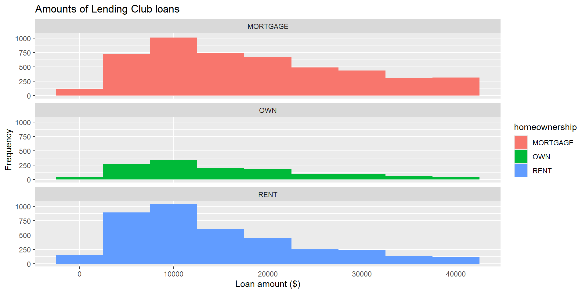
ggplot(loans, aes(x = loan_amount, fill = homeownership)) +
  geom_histogram(binwidth = 5000) +
  labs(
    x = "Loan amount ($)",
    y = "Frequency",
    title = "Amounts of Lending Club loans"
  ) +
  facet_wrap(~ homeownership, nrow = 3)

compare frequency - fewer people who take out loans own without a mortgage. regardless, it’s right skewed for all of them, more loan amounts under 10k than at 40k

Density plot

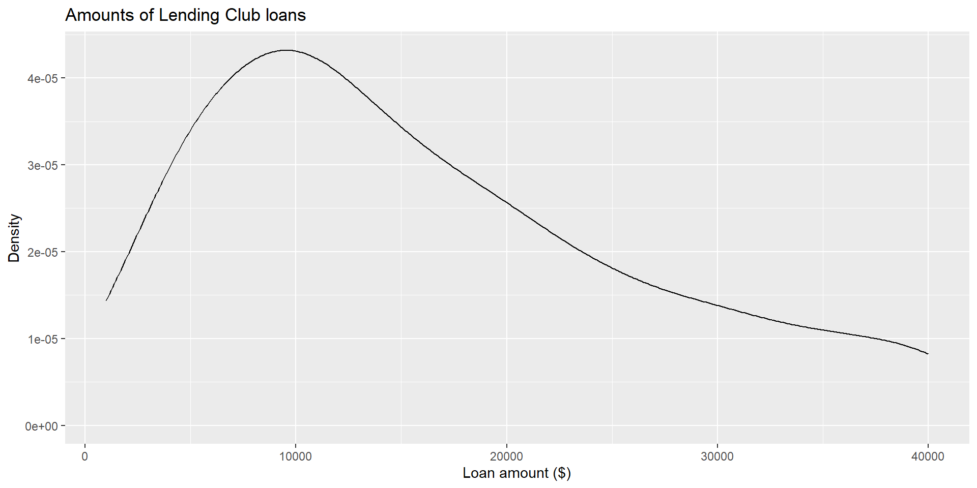
fitting a smooth curve on a histogram

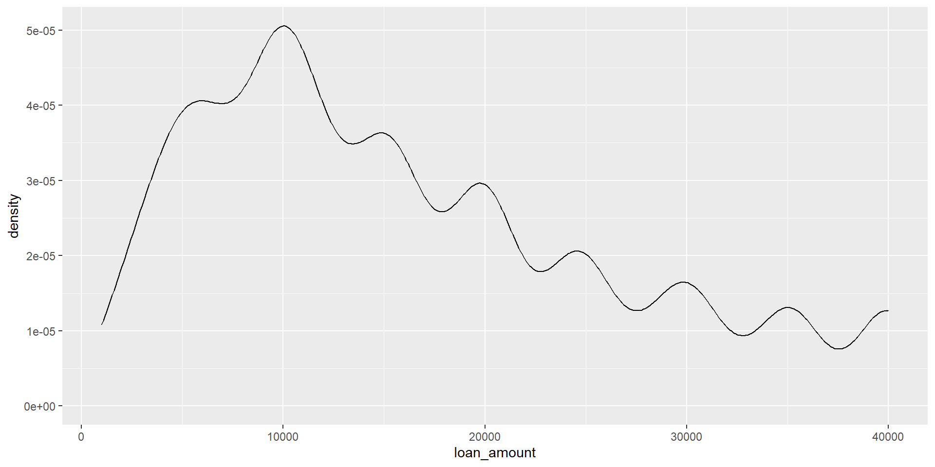
ggplot(loans, aes(x = loan_amount)) +
  geom_density()

Density plots and adjusting bandwidth

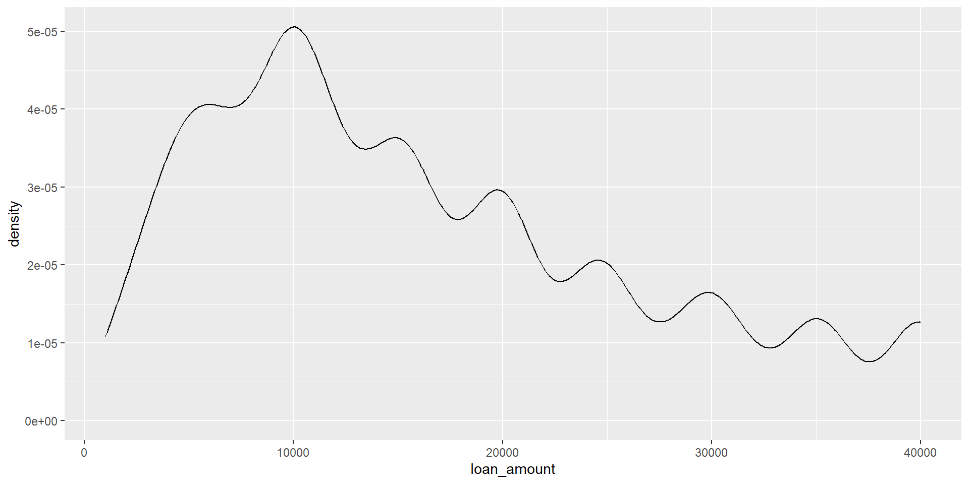
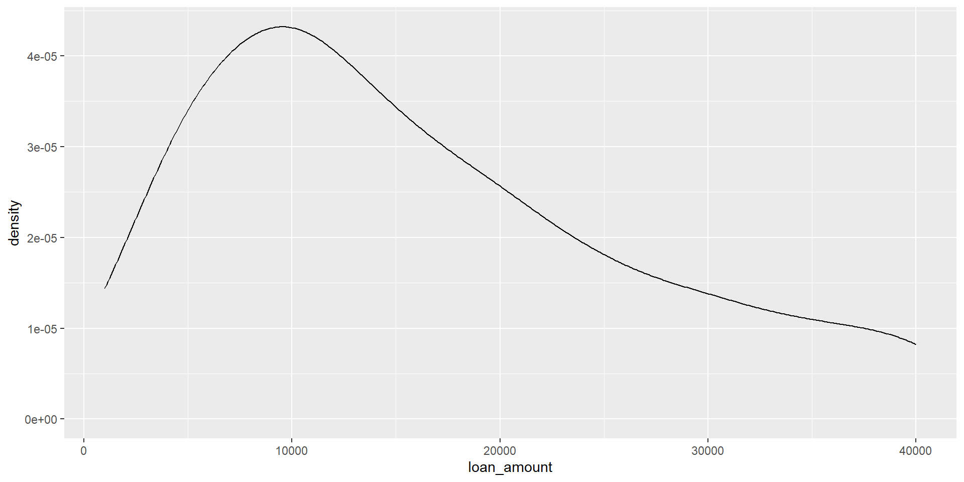
can adjust the smoothness - similar vibe to adjusting binwidth
higher number means you may loose out on a local max

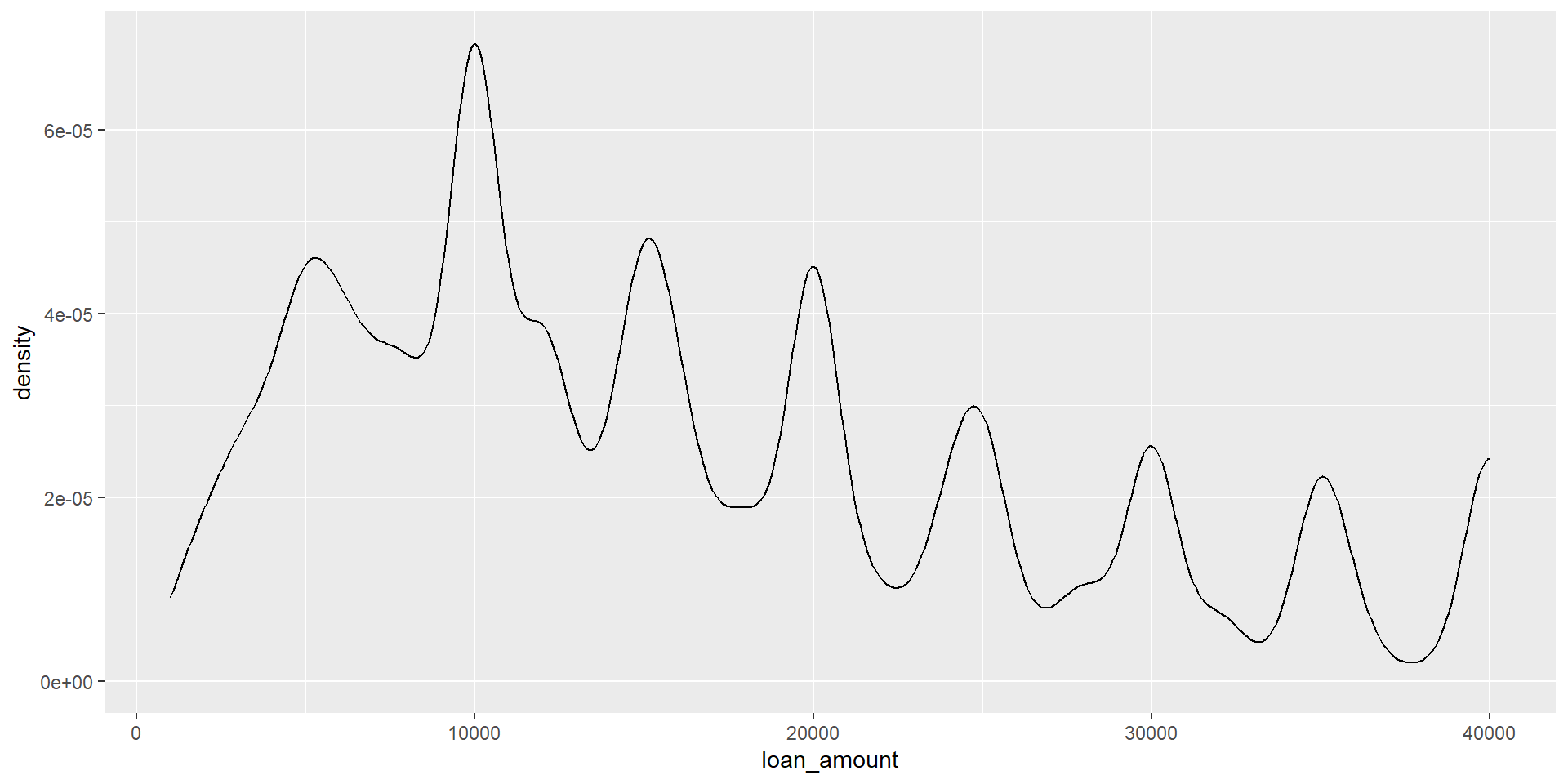
ggplot(loans, aes(x = loan_amount)) + geom_density(adjust = 0.5)
ggplot(loans, aes(x = loan_amount)) + geom_density(adjust = 1) # default bandwidth
ggplot(loans, aes(x = loan_amount)) + geom_density(adjust = 2)

Customizing density plots

ggplot(loans, aes(x = loan_amount)) +
  geom_density(adjust = 2) +
  labs(
    x = "Loan amount ($)",
    y = "Density",
    title = "Amounts of Lending Club loans"
  )

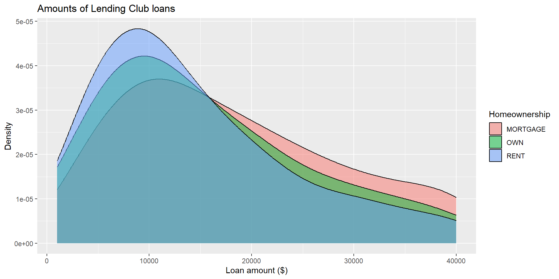
Adding a categorical variable

ggplot(loans, aes(x = loan_amount,
                  fill = homeownership)) +
  geom_density(adjust = 2,
               alpha = 0.5) +
  labs(
    x = "Loan amount ($)",
    y = "Density",
    title = "Amounts of Lending Club loans",
    fill = "Homeownership"
  )

Box plot

Box plot and outliers

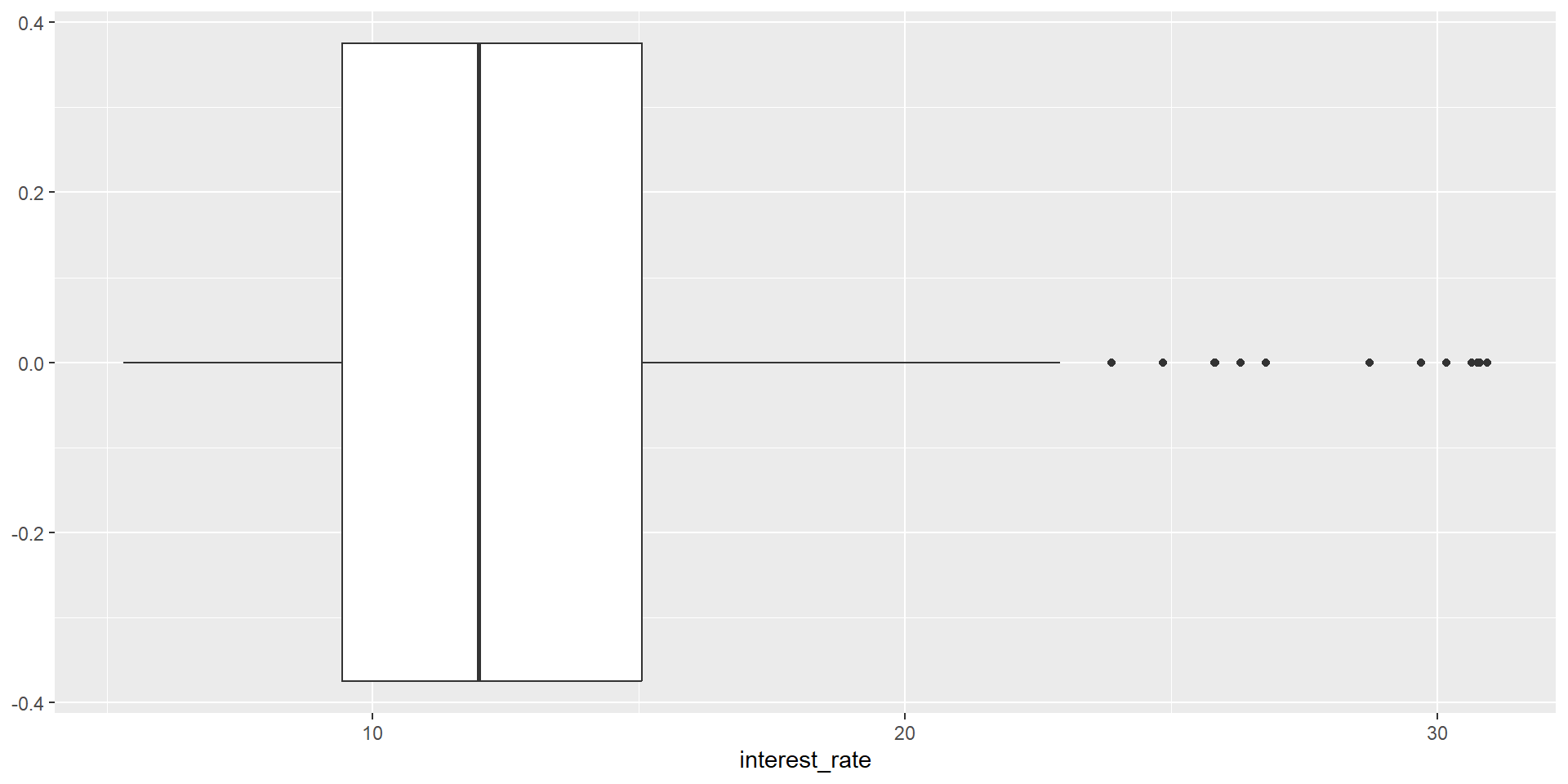
boxplots are good at uncovering outliers.
lot of people in the box, very few on the far right side

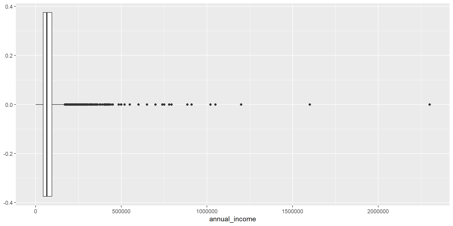
ggplot(loans, aes(x = annual_income)) +
  geom_boxplot()
ggplot(loans, aes(x = interest_rate)) +
  geom_boxplot()

same right skew, high end outliers, but fewer ppl are getting high interest rates

Customizing box plots

what’s up with the y axis? height of box?
explain theme
don’t always need to make these adjustments but it’s good to know these options are available for when you do

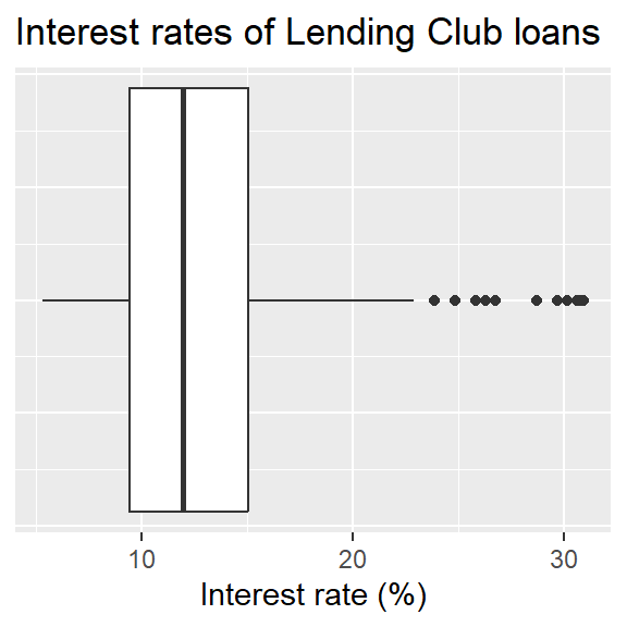
ggplot(loans, aes(x = interest_rate)) +
  geom_boxplot() +
  labs(
    x = "Interest rate (%)",
    y = NULL,
    title = "Interest rates of Lending Club loans"
  ) +
  theme(
    axis.ticks.y = element_blank(),
    axis.text.y = element_blank()
  )

Adding a categorical variable

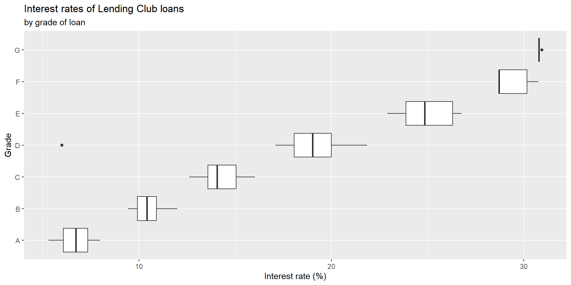
side by side boxplots are super common
grade is soemthing about the quality of the loan
to create this viz you add…

ggplot(loans, aes(x = interest_rate,
                  y = grade)) +
  geom_boxplot() +
  labs(
    x = "Interest rate (%)",
    y = "Grade",
    title = "Interest rates of Lending Club loans",
    subtitle = "by grade of loan"
  )

Relationships between numerical variables

Scatterplot

if you have higher income to debt ratio it may be harder for banks to want to loan to you and so you may end up with higher interest rate

note very few ppl with over 100% debt to income ratio. so something must be going on with them

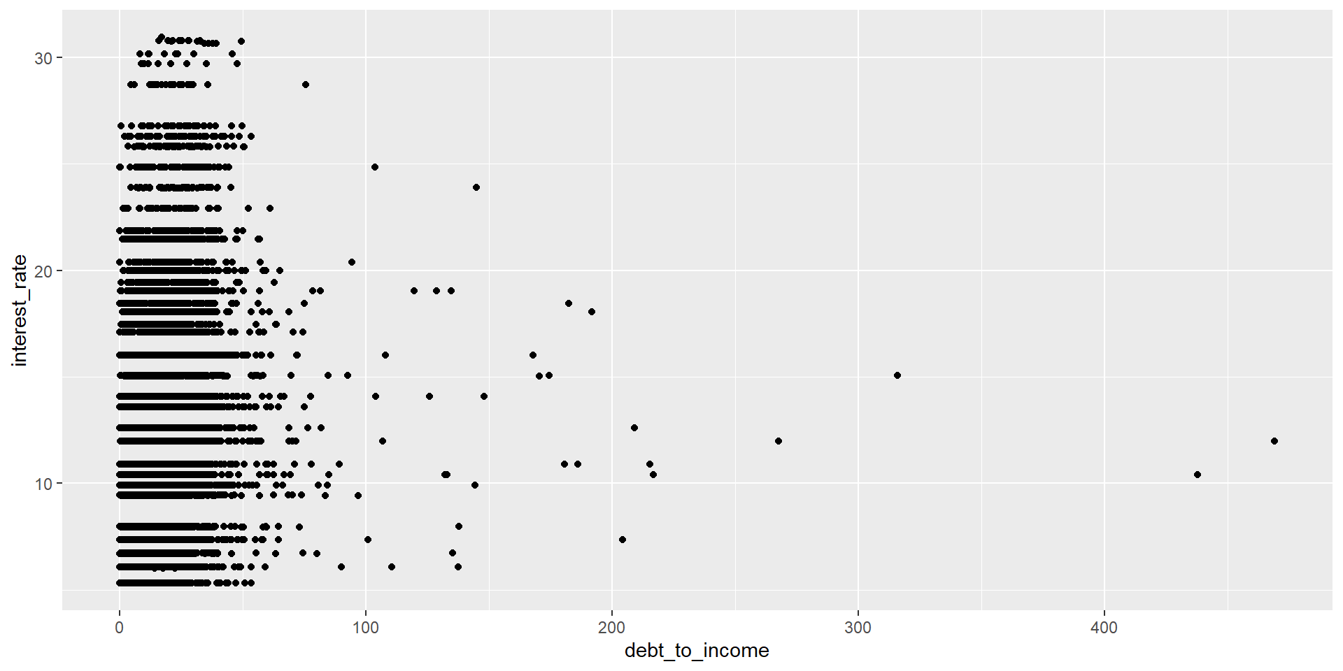
ggplot(loans, aes(x = debt_to_income, y = interest_rate)) +
  geom_point()

Hex plot

lot of oveplotting, so we can switch to geom_hex to create little 2d bins, where the color indicates how dense, or how many points are in that hex bin

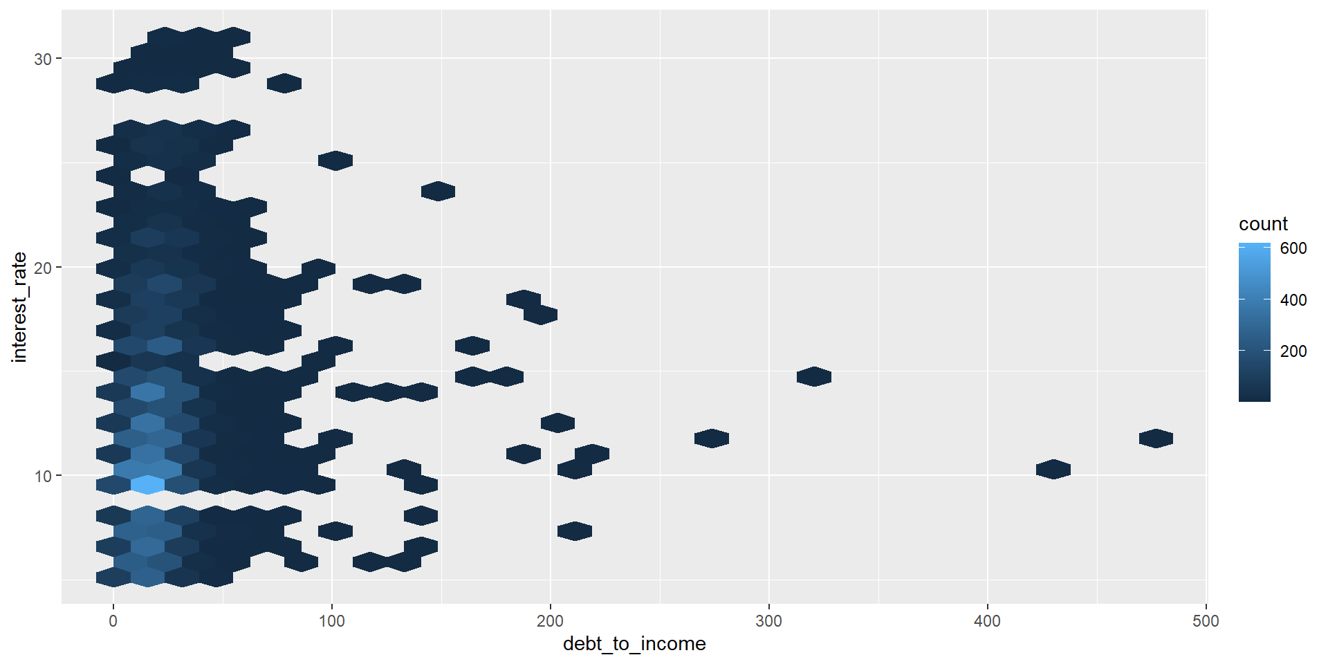
ggplot(loans, aes(x = debt_to_income, y = interest_rate)) +
  geom_hex()

Hex plot

lets filter the data set to only look at ppl whos debt to income ratio is less than 100%

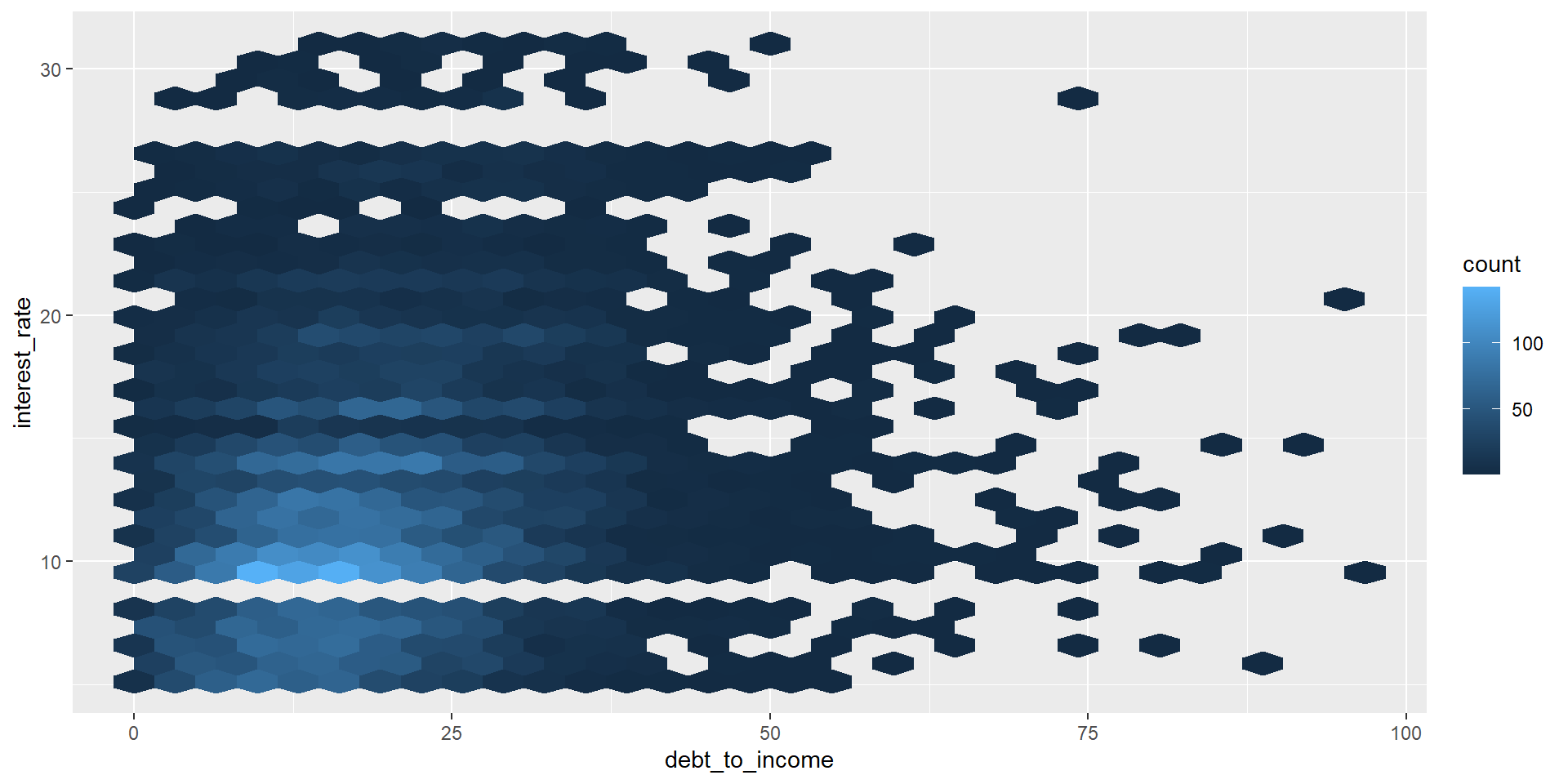
ggplot(loans %>% filter(debt_to_income < 100),
       aes(x = debt_to_income, y = interest_rate)) +
  geom_hex()

around 125 lots more loans being made at that level compared to others. because the hexbins are getting darker.

This page adapts material from Data Science in a Box (Unit 2, Deck 3: “Visualising numerical data”) by Mine Çetinkaya-Rundel, licensed under CC BY-SA 4.0. Source: tidyverse/datascience-box. Modified: reorganized into a Quarto revealjs deck; no dataset/package substitutions were needed for this lesson.