Linear Models

wk11-d01-linear-models

Dr. D

Chico State
DATA 385 - Fall 2026

November 3, 2026

Learning Materials

🎥 The language of models (27 min)

🎥 Fitting and interpreting models (30 min). Starts around slide 22

These slides mostly follow the videos, but are not direct code alongs.

library(tidyverse)
library(tidymodels) # new! Install it before first use.

New Packages

tidymodels: a collection of modeling packages that follow tidyverse principles. Today we use linear_reg(), fit(), tidy(), and predict().

Modeling

Two main purposes

• Prediction / classification
• Description / explanation

Can you think of examples of modeling for prediction vs. modeling for explanation?

Modeling cars

• What is the relationship between cars’ weights and their mileage?
• What is your best guess for a car’s MPG that weighs 3,500 pounds?

Modeling cars: describe

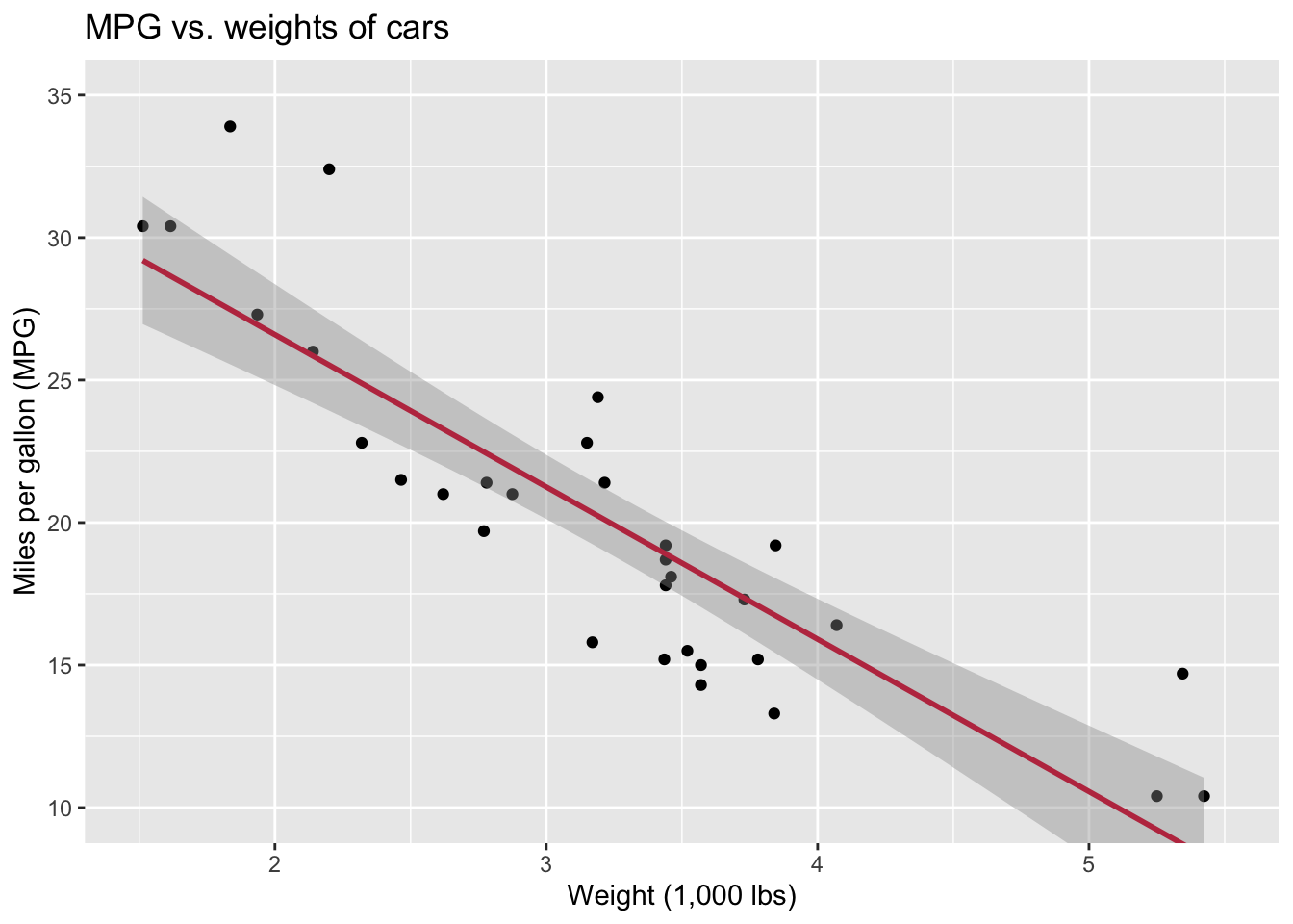
Describe: What is the relationship between cars’ weights and their mileage?

Modeling cars: predict

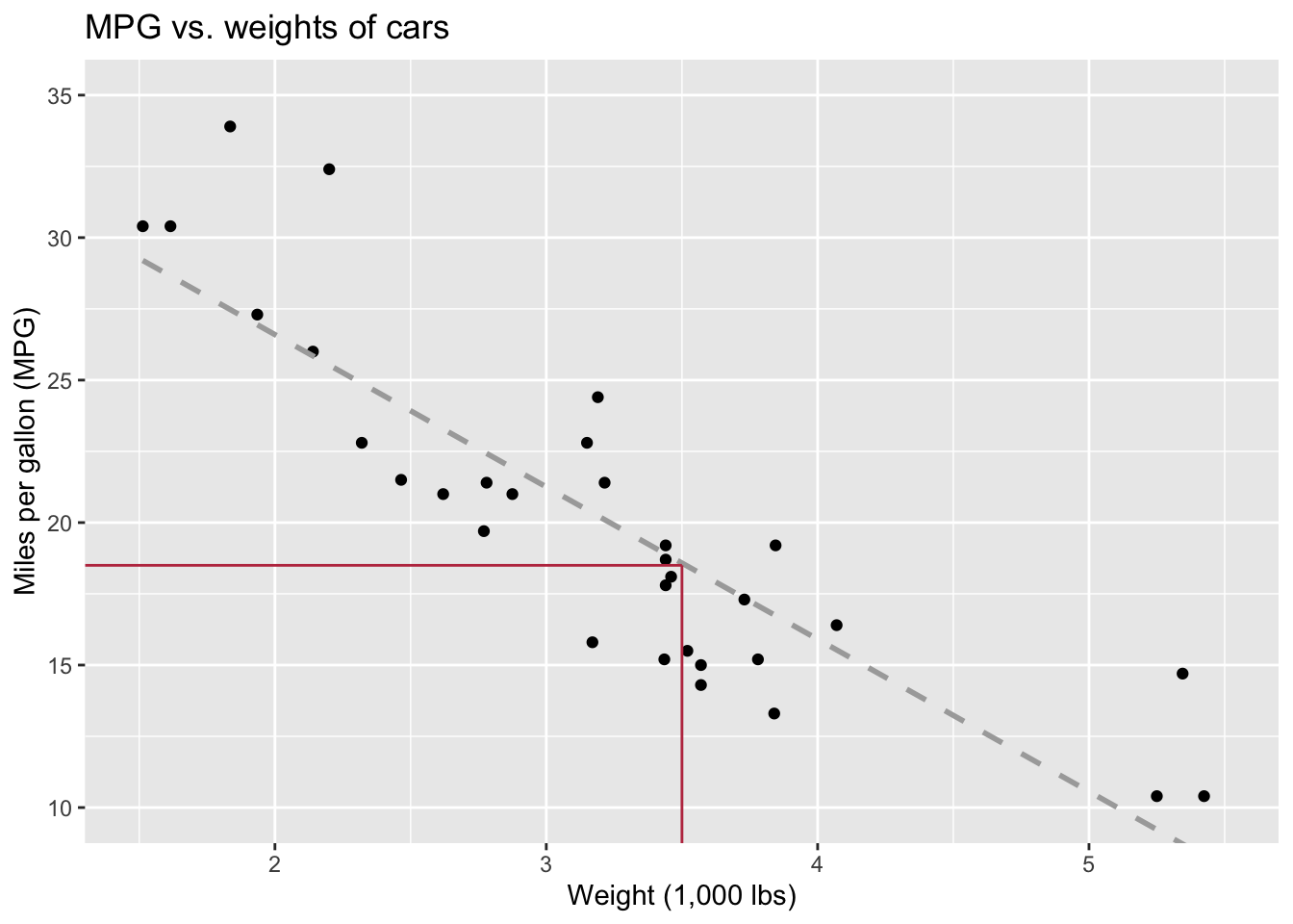
Predict: What is your best guess for a car’s MPG that weighs 3,500 pounds?

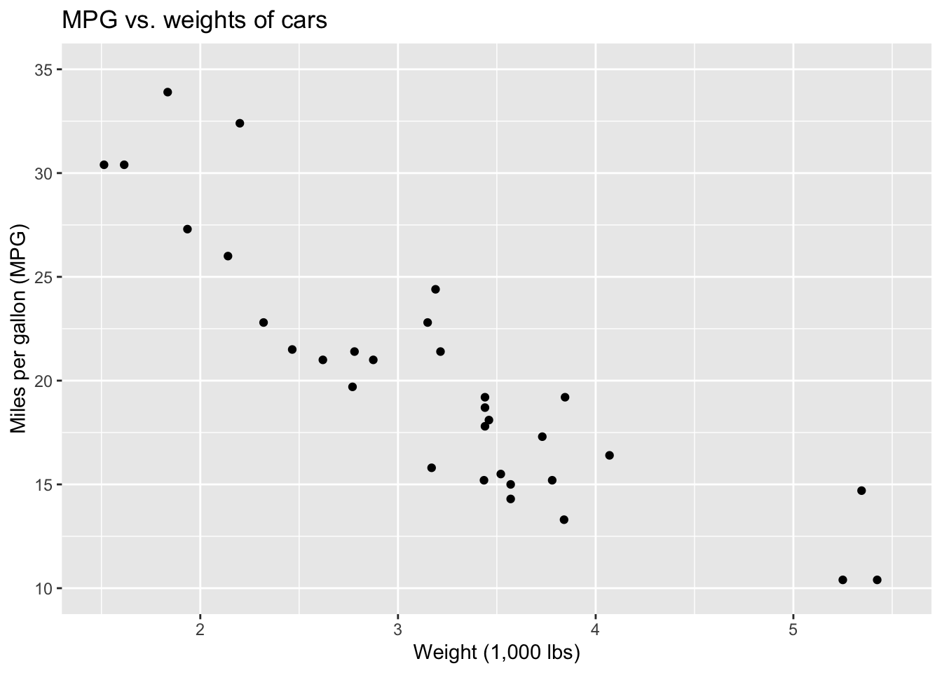
Why didn’t I use \(x=3500\)?

Modeling

• Use models to explain the relationship between variables and to make predictions
• For now we will focus on linear models (but there are many many other types of models too!)

Modeling vocabulary

• Explanatory variable
• Response variable
• Regression line
  • Slope
  • Intercept
• Correlation

Explanatory vs response

• response variable is the variable or characteristic of the data that we want to learn something about.
• explanatory variable is the variable whose effect on the response variable we are interested in establishing.

To identify the explanatory variable in a pair of variables, ask yourself which of the two is suspected of affecting the other.

Different words, same concept

Explanatory	Response	Field
\(x\)	\(y\)	statistics, mathematics
predictor, covariate	outcome	statistics, data science
independent	dependent	social sciences
regressor	regressand	econometrics
exposure, risk factor	outcome, endpoint	epidemiology, clinical trials
treatment		experiments, A/B tests
	criterion	psychology
input	output	machine learning, engineering
feature	target, label	machine learning

Predictor (explanatory variable)

                   mpg    wt
Mazda RX4         21.0 2.620
Mazda RX4 Wag     21.0 2.875
Datsun 710        22.8 2.320
Hornet 4 Drive    21.4 3.215
Hornet Sportabout 18.7 3.440
Valiant           18.1 3.460

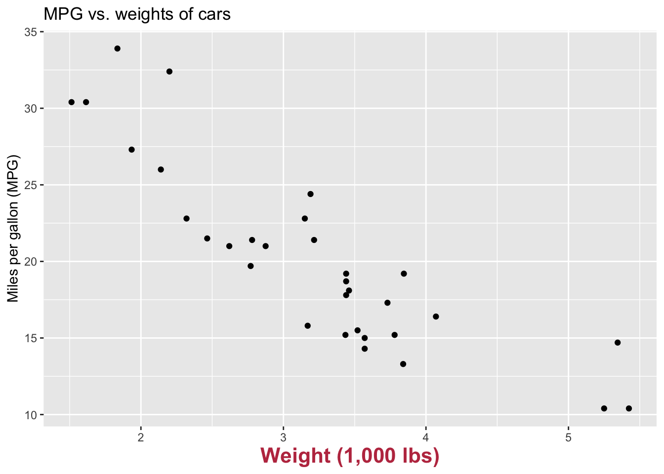
Explanatory goes on the x-axis

Outcome (response variable)

                   mpg    wt
Mazda RX4         21.0 2.620
Mazda RX4 Wag     21.0 2.875
Datsun 710        22.8 2.320
Hornet 4 Drive    21.4 3.215
Hornet Sportabout 18.7 3.440
Valiant           18.1 3.460

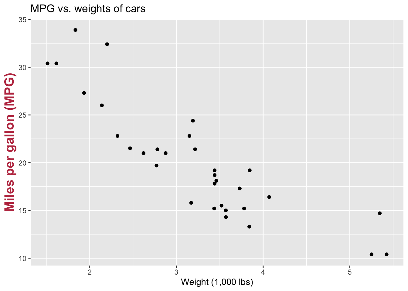
Response goes on the y-axis

Regression line

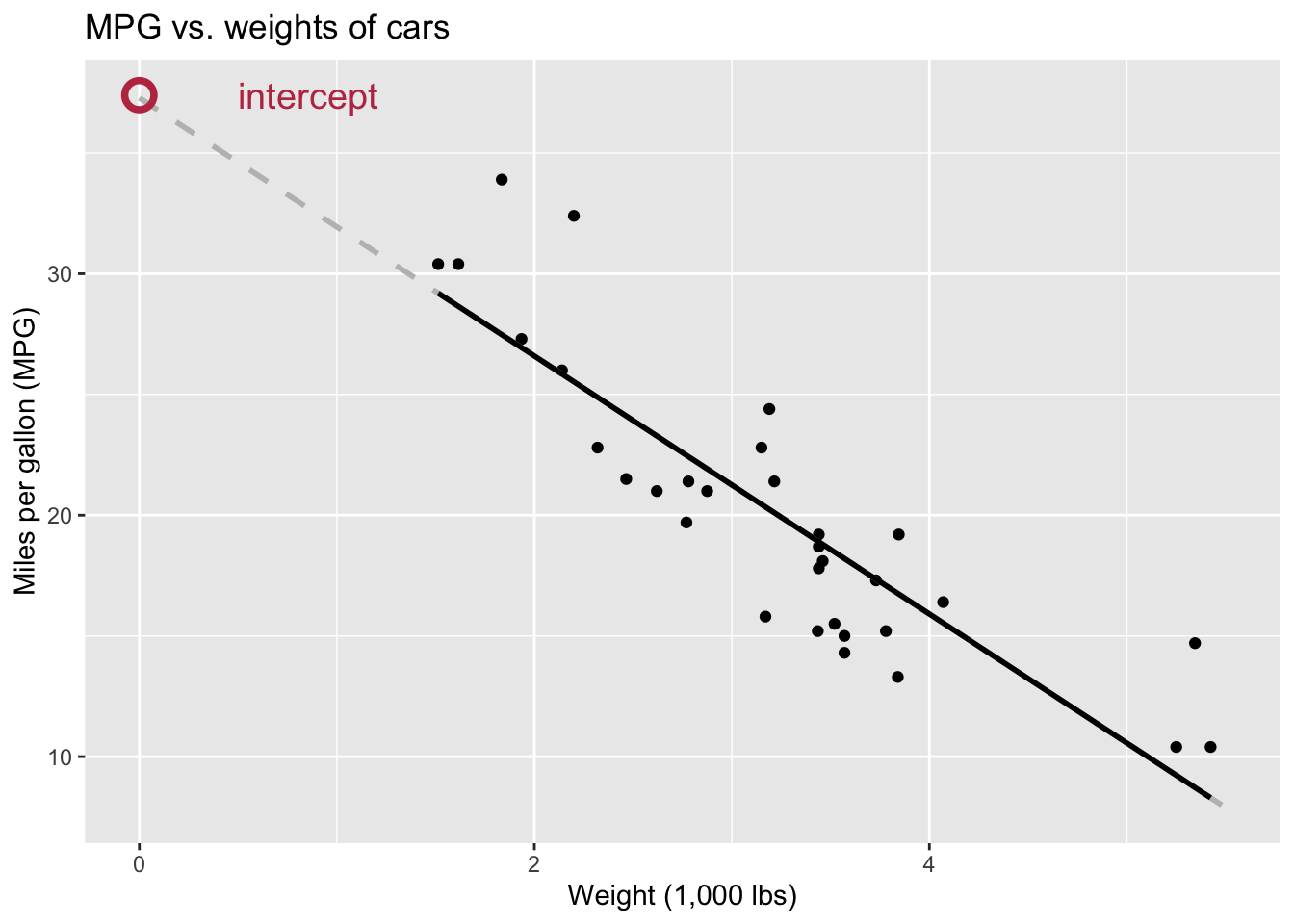
A linear model of the form \(y=mx+b\) can be used to describe the pattern of data.

Regression line: slope

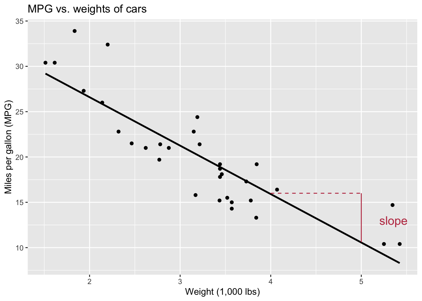
How much does \(y\) change when we increase \(x\) by 1 unit? (rise/run)

Regression line: intercept

If \(x=0\), what is the value of \(y\)? Often meaningless in context of the problem.

Correlation

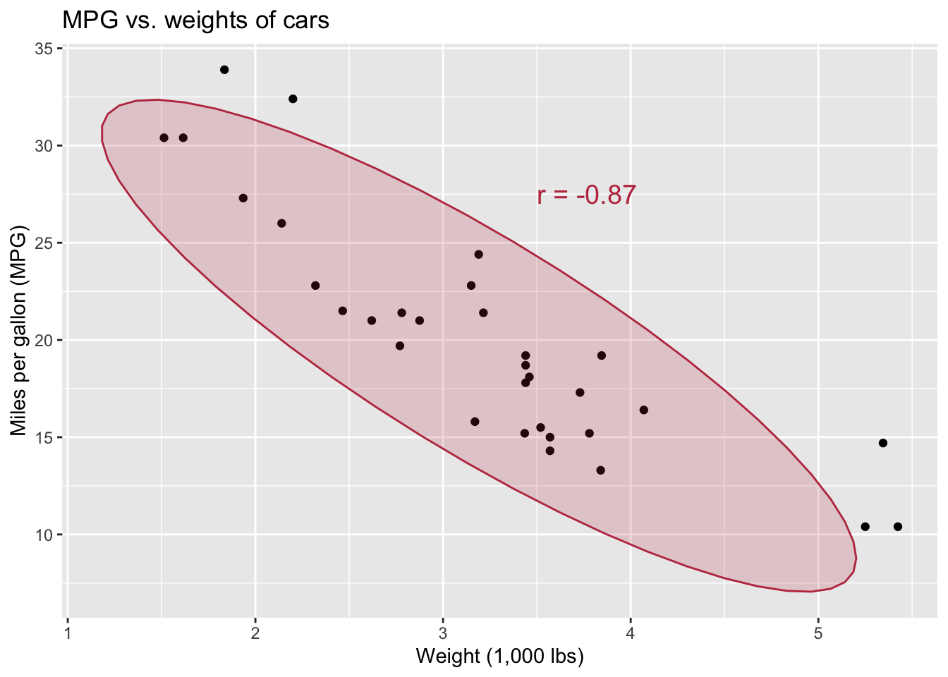
How tightly the points group around that line. How do X and Y covary together.

Correlation

• Ranges between -1 and 1.
• Same sign as the slope.

Guess the correlation

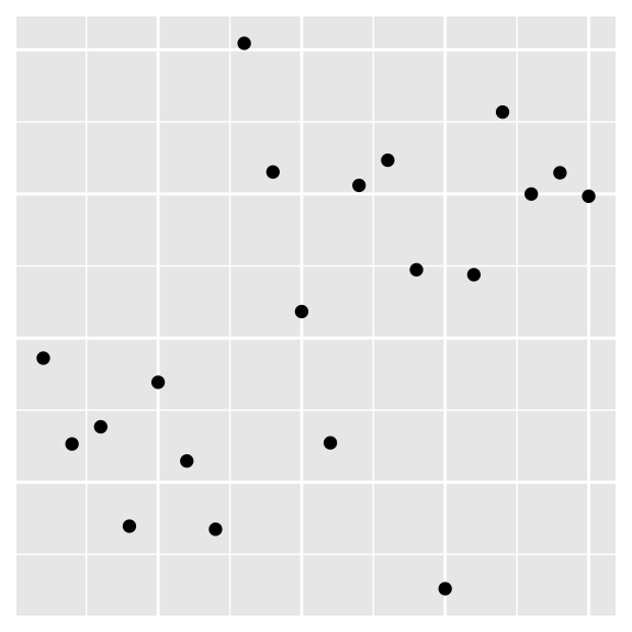
Which of these is the best guess for the correlation between the two variables?

• -0.95
• -0.53
• 0.00
• 0.25
• 0.80

Guess the correlation: answer

cor(df$x, df$y)

[1] 0.5007869

Visualizing the model

ggplot(mtcars, aes(x = wt, y = mpg)) +
  geom_point() +
  geom_smooth(method = "lm")

We’ve seen this type of plot before, now let’s get into the math behind how it’s made, and how it’s used for both description and prediction.

Linear regression with a single predictor

Regression model

A regression model is a function that describes the relationship between the observed data outcome, \(Y\), and the predictor, \(X\).

\[ \begin{aligned} \textbf{DATA} &= \textbf{MODEL} + \text{ERROR} \\[8pt] \mathbf{Y} &= \mathbf{f(X)} + \epsilon \\[8pt] \end{aligned} \]

ERROR is the part of variability in the observed data \(Y\) that is not explained by the model.

Regression model

\[ \begin{aligned} Y &= \color{#325b74}{\textbf{Model}} + \text{Error} \\[8pt] &= \color{#325b74}{\mathbf{f(X)}} + \epsilon \\[8pt] &= \color{#325b74}{\boldsymbol{\mu_{Y|X}}} + \epsilon \end{aligned} \]

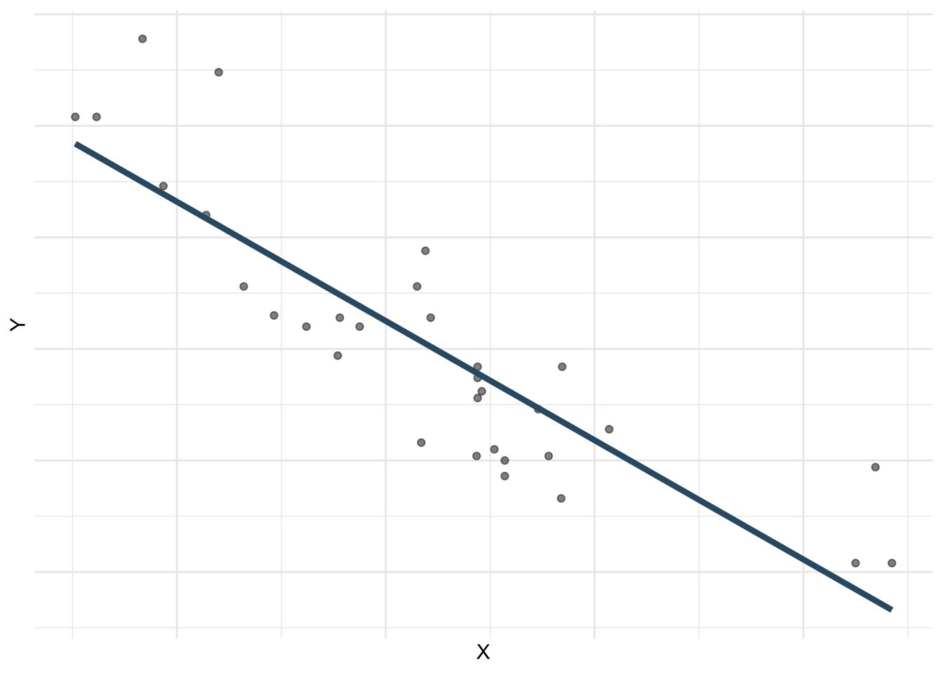
\({\boldsymbol{\mu_{Y|X}}}\) is the population mean of \(Y\), given a particular value for \(X\).

Simple linear regression

Use simple linear regression to model the relationship between a quantitative outcome (\(Y\)) and a single quantitative predictor (\(X\)): \[\Large{Y = \beta_0 + \beta_1 X + \epsilon}\]

• \(\beta_1\): True slope of the relationship between \(X\) and \(Y\)
• \(\beta_0\): True intercept of the relationship between \(X\) and \(Y\)
• \(\epsilon\): Error (residual)

Simple linear regression

If we knew the true model, we wouldn’t have to estimate it using data. But we don’t, so we do.

\[ \Large{\hat{Y} = b_0 + b_1 X} \]

• \(b_1\): Estimated slope of the relationship between \(X\) and \(Y\)
• \(b_0\): Estimated intercept of the relationship between \(X\) and \(Y\)
• No error term!

Choosing values for \(b_1\) and \(b_0\)

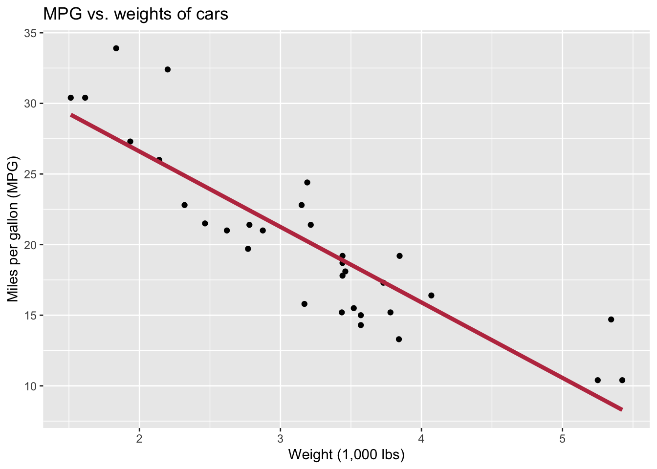
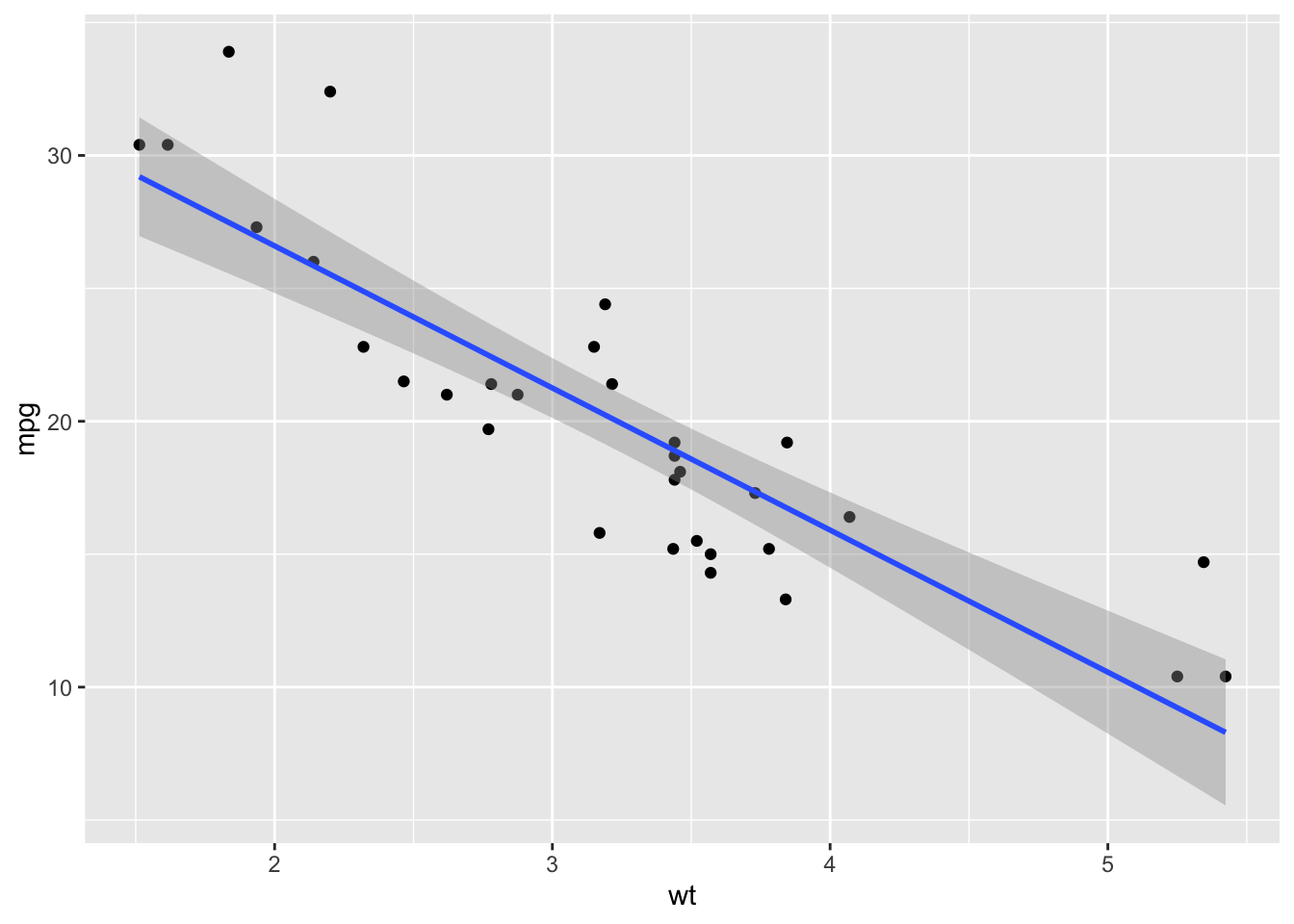
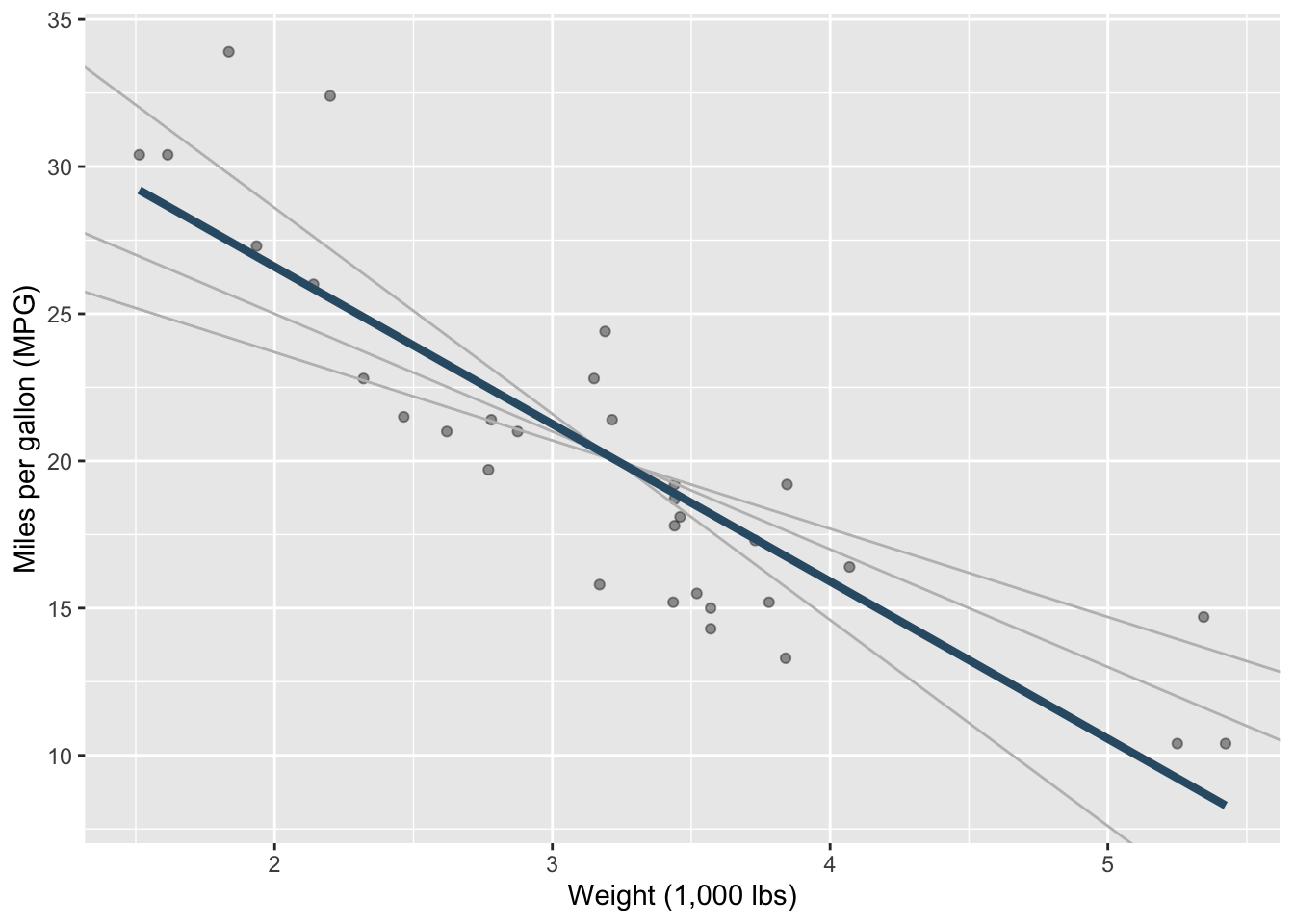
There are infinite number of lines (models) that could be fit. How do we find the model that best explains the data? How do we measure/quantify best?

Residuals (ERROR)

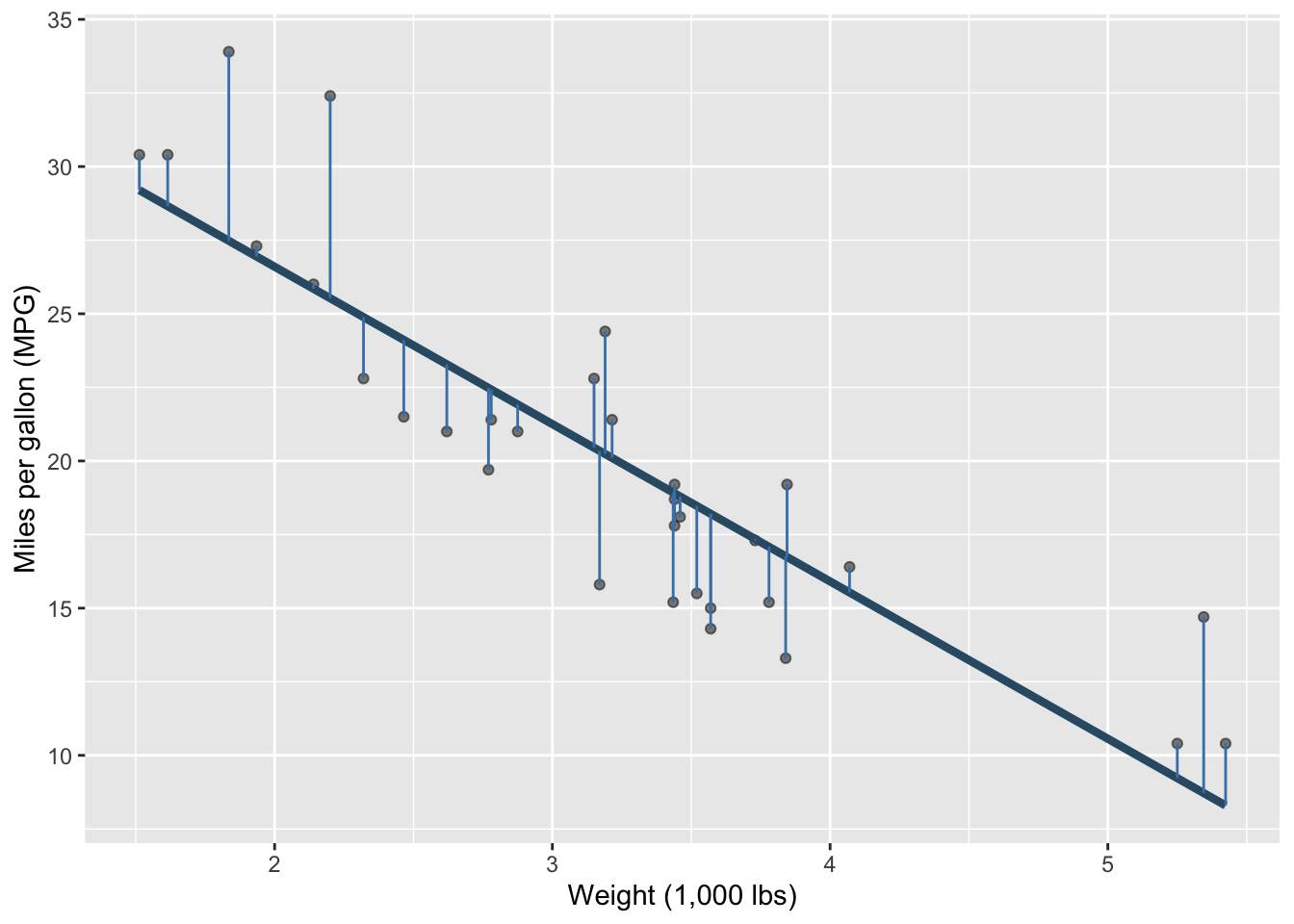
\[ \text{residual} = \text{observed} - \text{predicted} = y - \hat{y} \] How far away from the line (model) are the observed points?

Ordinary Least squares line

• The residual for the \(i^{th}\) observation is

\[ e_i = \text{observed} - \text{predicted} = y_i - \hat{y}_i \]

• The sum of squared residuals is

\[ e^2_1 + e^2_2 + \dots + e^2_n \]

• The least squares line is the one that minimizes the sum of squared residuals

I.e. The OLS is the “best fit” line.

Least squares line

cars_fit <- linear_reg() |>
  fit(mpg ~ wt, data = mtcars)

tidy(cars_fit)

# A tibble: 2 × 5
  term        estimate std.error statistic  p.value
  <chr>          <dbl>     <dbl>     <dbl>    <dbl>
1 (Intercept)    37.3      1.88      19.9  8.24e-19
2 wt             -5.34     0.559     -9.56 1.29e-10

Whatabout lm()? Same concept - linear_reg() is from the tidymodels package and integrates better into a modeling workflow that we’ll use in the next couple sections. Same math.

lm() –> linear_reg() + fit()

summary() –> tidy()

Slope and intercept

Properties of least squares regression

• The regression line goes through the center of mass point (the coordinates corresponding to average \(X\) and average \(Y\)): \(b_0 = \bar{Y} - b_1~\bar{X}\)
• Slope has the same sign as the correlation coefficient: \(b_1 = r \frac{s_Y}{s_X}\)
• Sum of the residuals is zero: \(\sum_{i = 1}^n e_i = 0\)
• Residuals and \(X\) values are uncorrelated

Interpreting the slope

Let \(y\) be MPG and \(x\) be weight (1,000 lbs).

\[\hat{y} = 37.3 - 5.34x\]

The slope is -5.34. Which of the following is the best interpretation of this value?

• For every additional 1,000 lbs of weight, MPG goes down by 5.34, on average.
• For every additional 1,000 lbs of weight, we expect MPG to be lower by 5.34, on average.
• For every additional 1,000 lbs of weight, MPG goes down by 5.34.
• For every additional 1 MPG, we expect weight to be lower by 5,340 lbs, on average.

Interpreting the intercept

Let \(y\) be MPG and \(x\) be weight (1,000 lbs).

\[\hat{y} = 37.3 - 5.34x\]

The intercept is 37.3. Which of the following is the best interpretation of this value?

• For cars that weigh 0 lbs, we expect MPG to be 37.3, on average.
• For cars with 0 MPG, we expect weight to be 37,300 lbs, on average.
• For every additional 1,000 lbs of weight, MPG goes up by 37.3.
• For cars with 0 MPG, we expect weight to be -5,340 lbs, on average.

Is the intercept meaningful?

✅ The intercept is meaningful in context of the data if

• the predictor can feasibly take values equal to or near zero or
• the predictor has values near zero in the observed data

🛑 Otherwise, it might not be meaningful!

Making predictions

What MPG does the model predict for a car that weighs 3,500 lbs?

\[\hat{y} = 37.3 - 5.34(3.5) \approx 18.6\]

# make a new data set for the new value of x. 
# must have same variable name as used in the model
new_car <- tibble(wt = 3.5) 

cars_fit |>
  predict(new_data = new_car)

# A tibble: 1 × 1
  .pred
  <dbl>
1  18.6

Extrapolation

What about a car that weighs 8,000 lbs?

heavy_car <- tibble(wt = 8)

cars_fit |>
  predict(new_data = heavy_car)

# A tibble: 1 × 1
  .pred
  <dbl>
1 -5.47

mtcars |>
  summarize(min_wt = min(wt), max_wt = max(wt))

  min_wt max_wt
1  1.513  5.424

Predicting outside the range of the observed data is extrapolation. The model has no data there, so don’t trust it.

Categorical predictors

Models with categorical predictors

• When the categorical predictor has many levels, they’re encoded to indicator variables (aka “dummy” variables)
• The first level of the categorical variable is the baseline level. In a model with one categorical predictor, the intercept is the predicted value of the outcome for the baseline level (x = 0).
• Each slope coefficient describes the difference between the predicted value of the outcome for that level of the categorical variable compared to the baseline level.

MPG by transmission

am is coded 0 = automatic, 1 = manual. Make it a categorical variable.

mtcars_trans <- mtcars |>
  mutate(transmission = if_else(am == 0, "automatic", "manual"))

ggplot(mtcars_trans, aes(x = transmission, y = mpg)) + geom_boxplot()

Mean MPG by transmission

mtcars_trans |>
  group_by(transmission) |>
  summarize(mean_mpg = mean(mpg))

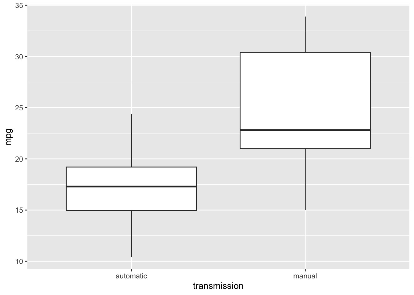
# A tibble: 2 × 2
  transmission mean_mpg
  <chr>           <dbl>
1 automatic        17.1
2 manual           24.4

The mean is a model. We are using \(\bar{y}\) to estimate \(\mu\). But we can build a better model by incorporating information from another variable, \(x\) (transmission).

Fit the model

trans_fit <- linear_reg() |>
  fit(mpg ~ transmission, data = mtcars_trans)

tidy(trans_fit)

# A tibble: 2 × 5
  term               estimate std.error statistic  p.value
  <chr>                 <dbl>     <dbl>     <dbl>    <dbl>
1 (Intercept)           17.1       1.12     15.2  1.13e-15
2 transmissionmanual     7.24      1.76      4.11 2.85e- 4

Which transmission is the baseline? How do the intercept and slope relate to the group means on the previous slide?

Interpret the estimates

Let \(y\) be MPG, and let \(x = 1\) for manual cars and \(x = 0\) for automatic cars.

\[\hat{y} = 17.15 + 7.24x\]

• Baseline: automatic. It comes first alphabetically, so it doesn’t get its own row in the output.
• transmissionmanual is the indicator variable \(x\) in the equation.

Plug in each group:

• Automatic (\(x = 0\)): \(\hat{y} = 17.15 + 7.24(0) = 17.15\)
• Manual (\(x = 1\)): \(\hat{y} = 17.15 + 7.24(1) = 24.39\)

The intercept is the mean MPG for the baseline group. The slope is the difference between the group means: \(24.39 - 17.15 = 7.24\).

Acknowledgements & Credits

Note

This deck adapts material from STA 199: Introduction to Data Science and Statistical Thinking (Duke University, Fall 2025) by Mine Çetinkaya-Rundel and Mary Knox: Lecture 15, “Language of models,” and Lecture 16, “Linear models with a single predictor.” Source: sta199-f25/sta199-f25.github.io. The videos linked in Setup are from Data Science in a Box (Unit 4, Decks 1 and 2) by Mine Çetinkaya-Rundel, licensed under CC BY-SA 4.0. Modified: combined the two lectures into one deck starting at Lecture 15’s Modeling section; replaced the fandango movie scores data with mtcars; replaced Wooclap polls with discussion questions; dropped the warm-ups, the algorithmic bias section, the blood pressure study, the Tesla example, the gt tables, and the penguins recap; added prediction, extrapolation, and a transmission example for binary predictors.