Intro to Data Science

Welcome Aboard

Dr. Robin Donatello

Chico State
DATA 385 - Fall 2026

August 25, 2026

Hello world!

Meet Dr. D

  • Professor of Statistics (and Data Science)
  • Proud alum from Butte College & Chico State (BS Biology, BS Statistics, minor in Chemistry)
  • Doctorate in Public Health - Biostatisics from UCLA
  • Director of the Wildcat Data Hub and the Data Science Initiative at Chico State
  • Data Manager at the Center for Healthy Communities
  • Pitbull mamma, veggie gardner, and gamer (TTRPG and video games)

Office: Holt 202 Office hours:

  • Mon 1-2pm, T/R 2-3pm in Holt 202
  • Wed 1-3pm at Community Coding
  • By appointment (booking link in Canvas, on syllabus and on my website)

Meet each other!

Please share with at least two classmates…

  • Your name
  • Your year
  • Where you’re from
  • What you did this past summer
  • What you hope to get out of this course

Class Expectations

Highly active (on your part)

  • Normally day 1 is “go over the syllabus”. I talk about what the class is like, you listen passively.

  • We’re going to flip that and first see what Data Science can be like with an example

  • And then you’re going to work through HW0 and start investigating how this class is run/put together.

  • Short short version - all materials are on the class website.

Meet data science

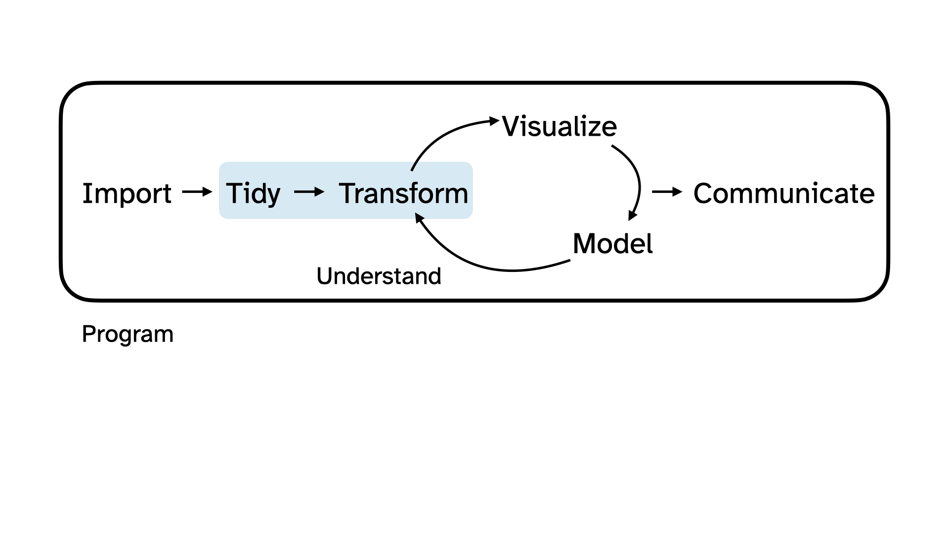
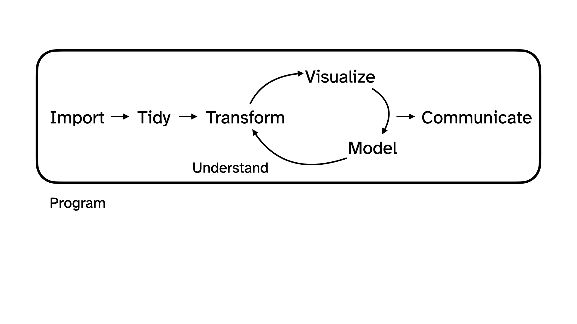
Data science cycle: Import, tidy, transform, visualize, model, communicate.

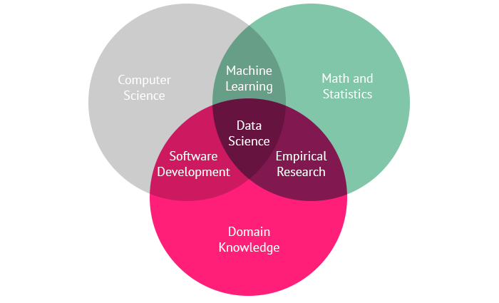
Management circle diagram.

  • Data science is an exciting discipline that allows you to turn raw data into understanding, insight, and knowledge.
  • It’s not just Stats, not just CS, and not just business (or some other domain) but a blend of all three.
  • We’re going to learn to do this in a modern, reproducible, and tidy way – more on that later!
  • This is a course on introduction to data science, with an emphasis on learning about our world through data.

Let’s do some data science!

Data Collection

  • Yesterday we collected some data from you!
  • Today we’re going to explore that data together, following the data science cycle.
  • Didn’t take it yet? Scan the QR code and do it now!

QR code linking to the survey.

Beginning the data science cycle

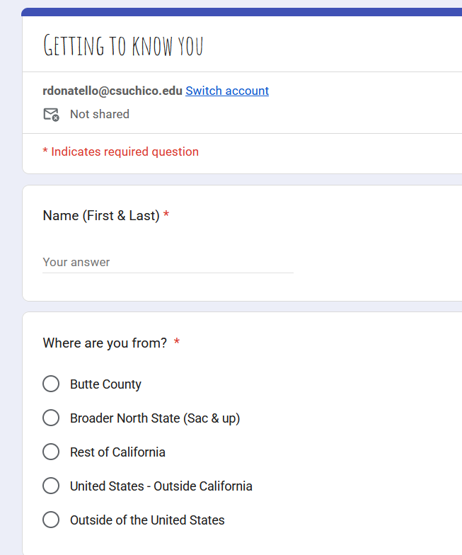
Screenshot of Getting to know you survey on Google.

  • You took a survey, built in Google Forms:

  • We want to explore that data and get to know you!

Load some packages

More on what packages are on Thursday, but in a nutshell “get your tools out of the toolbox”:

Code
library(tidyverse)   # for data wrangling and visualization
library(scales)      # for better axis labels
library(tidytext)    # for handling text data
library(ggwordcloud) # for the learn-best word cloud
library(zipcodeR)    # for the hometown map
library(maps)        # also for mapping
library(ggpubr)      # for better density plot
library(googlesheets4) # to get data from Google Sheets
library(sjPlot)      # also nice barcharts

You can click the arrow to see the code that was used.

Import

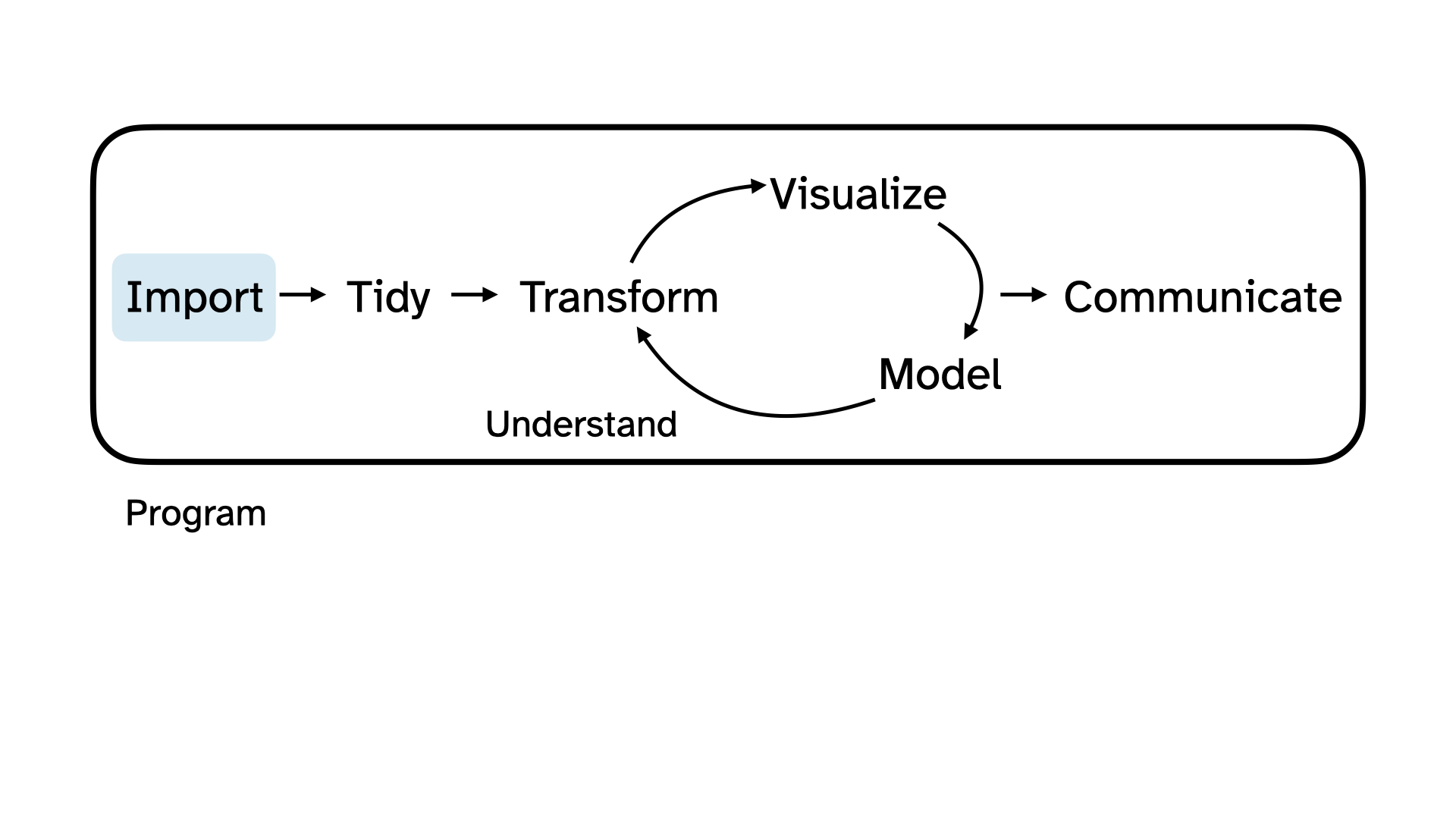
Data science cycle: Import, tidy, transform, visualize, model, communicate. Import is highlighted.

Import the data

We could download the data and save it as a csv file on our computer, edit out the student names, name it survey-anonymized.csv and save it in a folder called data. Then we would import it into R using the read_csv() function:

Code
survey <- read_csv(here::here("notes/data/survey-anonymized.csv"))

Import the data - Live connection

Alternatively, we can authorize R to directly read the Google Sheet that holds the responses from the Google Form you filled out.

Code
survey <- read_sheet("https://docs.google.com/spreadsheets/d/1R4_afqSB6KXD9HwfYP-wjMqvwxiDTGEMATmWmkqqXig")

Take a peek 👀 at the data

Code
survey
# A tibble: 21 × 7
   zipcode stats_experience                     programming_experience
     <dbl> <chr>                                <chr>                 
 1   95618 Yes, I have taken another college c… A lot — I use program…
 2   95129 Yes, I have taken another college c… Some — I’ve worked on…
 3   95932 Yes, I have taken another college c… Some — I’ve worked on…
 4   94526 Yes, I have taken a high school sta… A lot — I use program…
 5   95973 Yes, I have taken a high school sta… Some — I’ve worked on…
 6   94550 Yes, I have taken another college c… A lot — I use program…
 7   96080 Yes, I have taken another college c… Some — I’ve worked on…
 8   94510 Yes, I have taken another college c… Some — I’ve worked on…
 9   96007 Yes, I have taken another college c… Some — I’ve worked on…
10   92672 Yes, I have taken another college c… A lot — I use program…
# ℹ 11 more rows
# ℹ 4 more variables: programming_language <chr>,
#   data_interests <chr>, learn_best <chr>, commute_minutes <dbl>

Different data types require different approaches.

Multiple choice

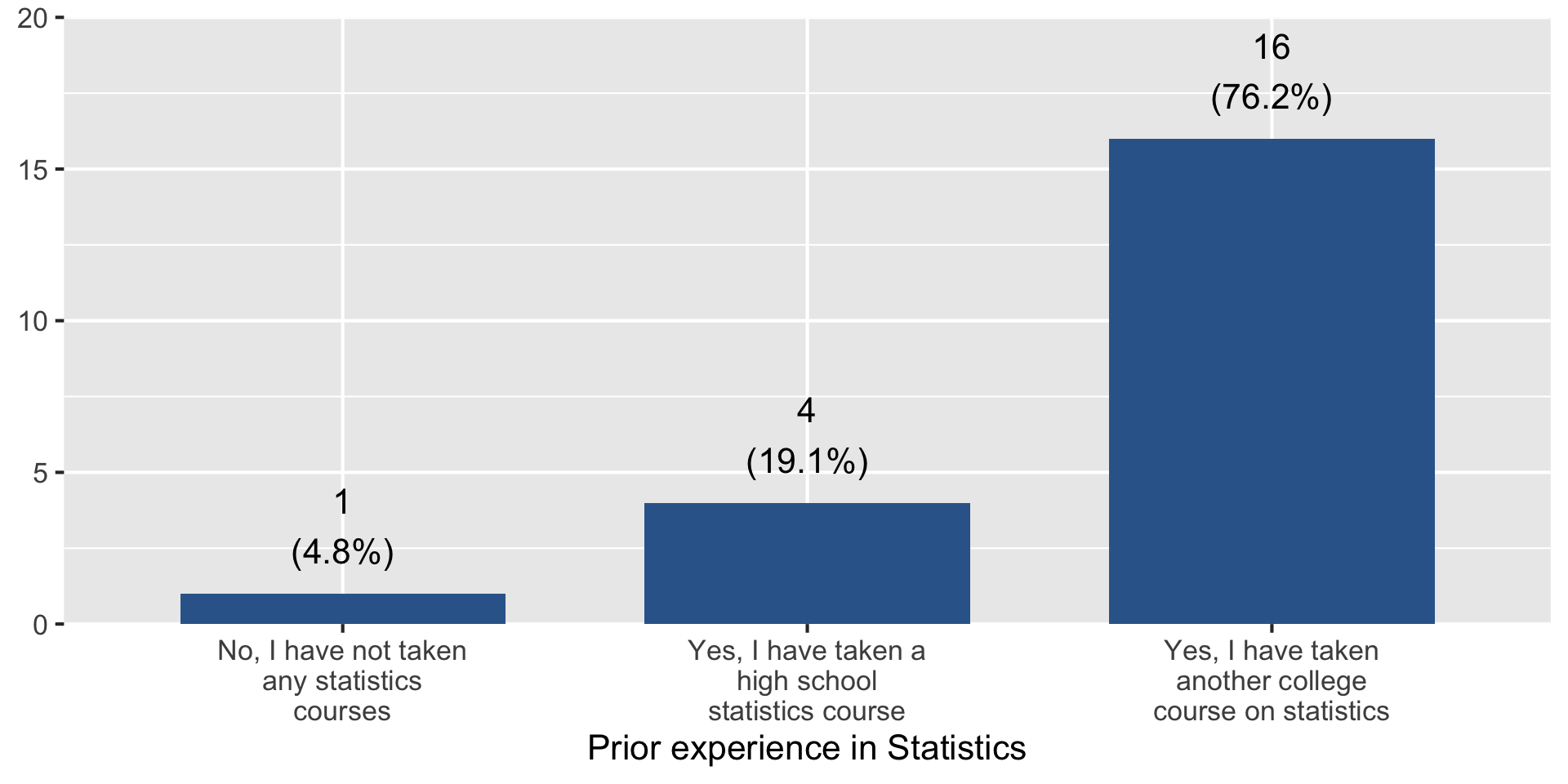
We asked you the following multiple-choice question where you could only pick one option:

Tip

Have you taken any statistics courses before?

  • Yes, I have taken another college course on statistics
  • Yes, I have taken a high school statistics course
  • No, I have not taken any statistics courses

Visualize

One way to make sense of data collected via a question like this is to visualize it.

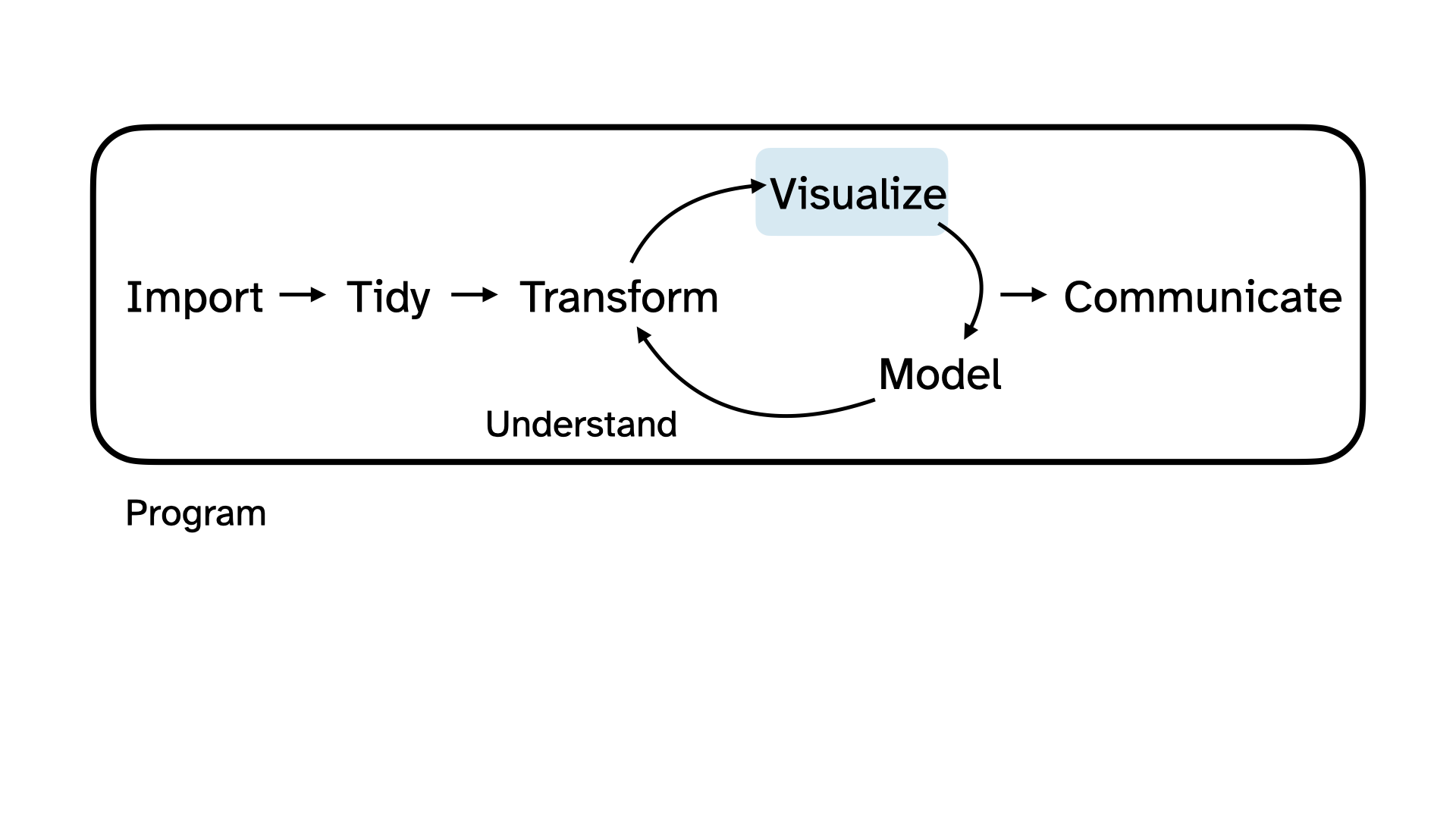
Data science cycle: Import, tidy, transform, visualize, model, communicate. Visualize is highlighted.

Visualize

Code
plot_frq(survey$stats_experience) + 
  xlab("Prior experience in Statistics")

Multiple Choice (cont.)

Tip

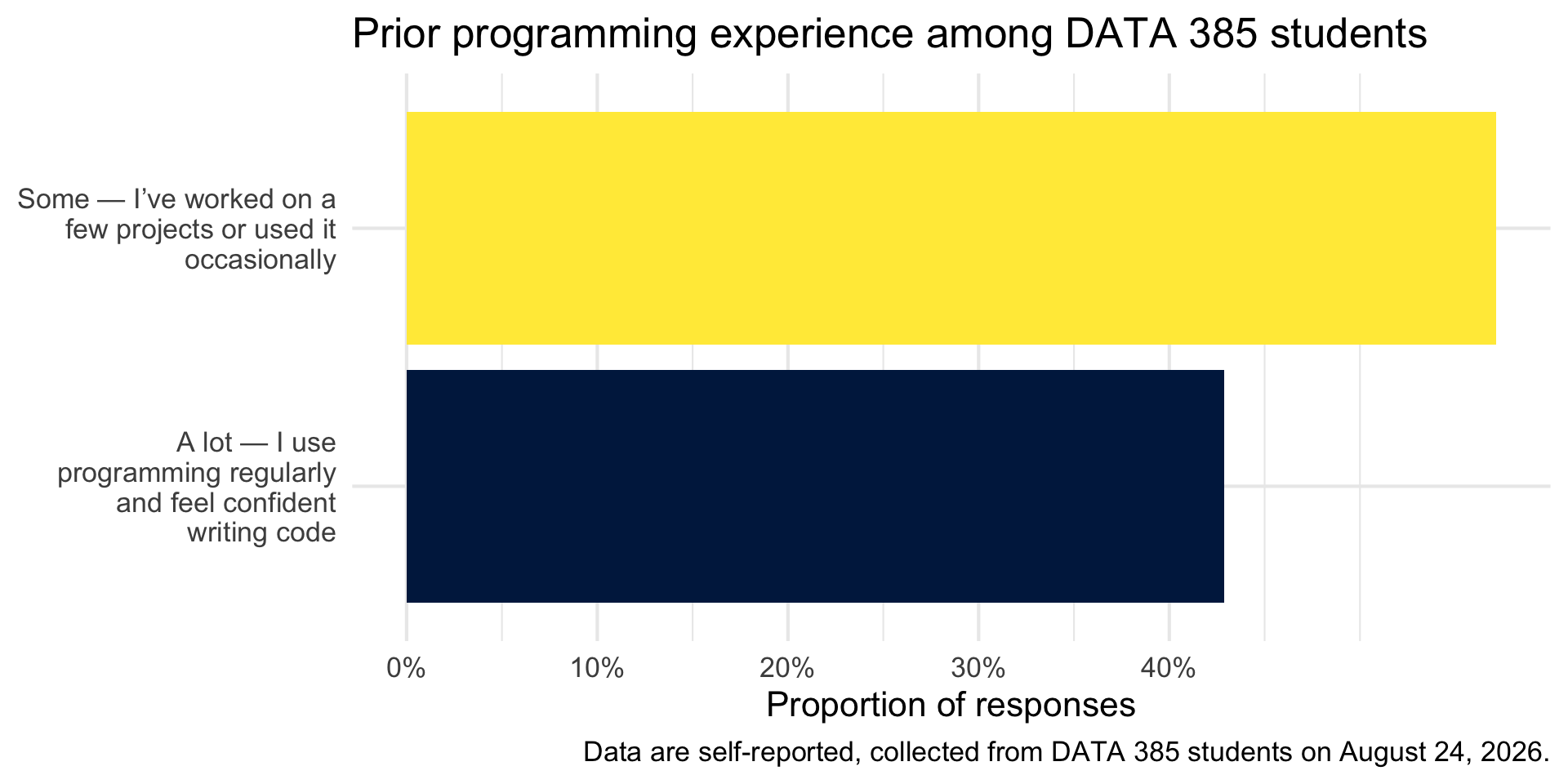
How much experience do you have with programming?

  • None
  • A little — I’ve written a few lines or done small exercises
  • Some — I’ve worked on a few projects or used it occasionally
  • A lot — I use programming regularly and feel confident writing code

Visualize

Code
survey |>
  count(programming_experience) |>
  mutate(prop = n / sum(n)) |>
  ggplot(aes(y = fct_reorder(programming_experience, prop), x = prop, fill = prop))+
  geom_col(show.legend = FALSE) +
  scale_y_discrete(labels = label_wrap(25)) +
  scale_x_continuous(labels = percent_format(accuracy = 1), breaks = c(0, 0.1, 0.2, 0.3, 0.4)) +
  scale_fill_viridis_c(option = "E") +
  labs(
    title = "Prior programming experience among DATA 385 students",
    y = NULL,
    x = "Proportion of responses"
  ) +
  labs(
    caption = "Data are self-reported, collected from DATA 385 students on August 24, 2026."
  ) +
  theme_minimal(base_size = 16)

Mark all that apply

We also asked you the following multiple-answer question where you could as many options as you liked:

Tip

What types of data interest you?

  • Crime
  • Economics
  • Education
  • Entertainment (e.g., books, movies, music)
  • Environment/Climate
  • Health (e.g., social determinants of health, medical)
  • Politics
  • Sports
  • Other
  • No preference

Peek at the data 👀

Code
survey |>
  select(data_interests)
# A tibble: 21 × 1
   data_interests                                                     
   <chr>                                                              
 1 - Crime, - Economics, - Environment/Climate, - Politics            
 2 - Economics, - Sports                                              
 3 - No preference                                                    
 4 - Crime, - Economics, - Education, - Entertainment (e.g., books, m…
 5 - No preference                                                    
 6 - Economics, - Education, - Health (e.g., social determinants of h…
 7 - Economics, - Health (e.g., social determinants of health, medica…
 8 - Crime, - Economics, - Environment/Climate, - Politics, - Sports  
 9 - Crime, - Education, - Entertainment (e.g., books, movies, music)…
10 - Economics, - Entertainment (e.g., books, movies, music), - Polit…
# ℹ 11 more rows
What do you notice?

Tidy + Transform

Before we can visualize this variable, we need to tidy and transform it.

Data science cycle: Import, tidy, transform, visualize, model, communicate. Tidy and transform are highlighted.

Tidy + Transform

Code
survey |>
  # remove text in parentheses
  mutate(data_interests = str_remove_all(data_interests, "\\s*\\(.*?\\)|\\s*-\\s*")) |>
  # separate into multiple rows for each interest, using comma as delimiter
  separate_longer_delim(data_interests, delim = ",") |>
  mutate(data_interests = trimws(data_interests)) |>
  count(data_interests, sort = TRUE) |>
  mutate(prop = n / sum(n))
# A tibble: 10 × 3
   data_interests          n   prop
   <chr>               <int>  <dbl>
 1 Economics              14 0.182 
 2 Crime                  10 0.130 
 3 Health                 10 0.130 
 4 Sports                 10 0.130 
 5 Politics                9 0.117 
 6 Environment/Climate     8 0.104 
 7 Education               6 0.0779
 8 Entertainment           6 0.0779
 9 No preference           2 0.0260
10 Other                   2 0.0260

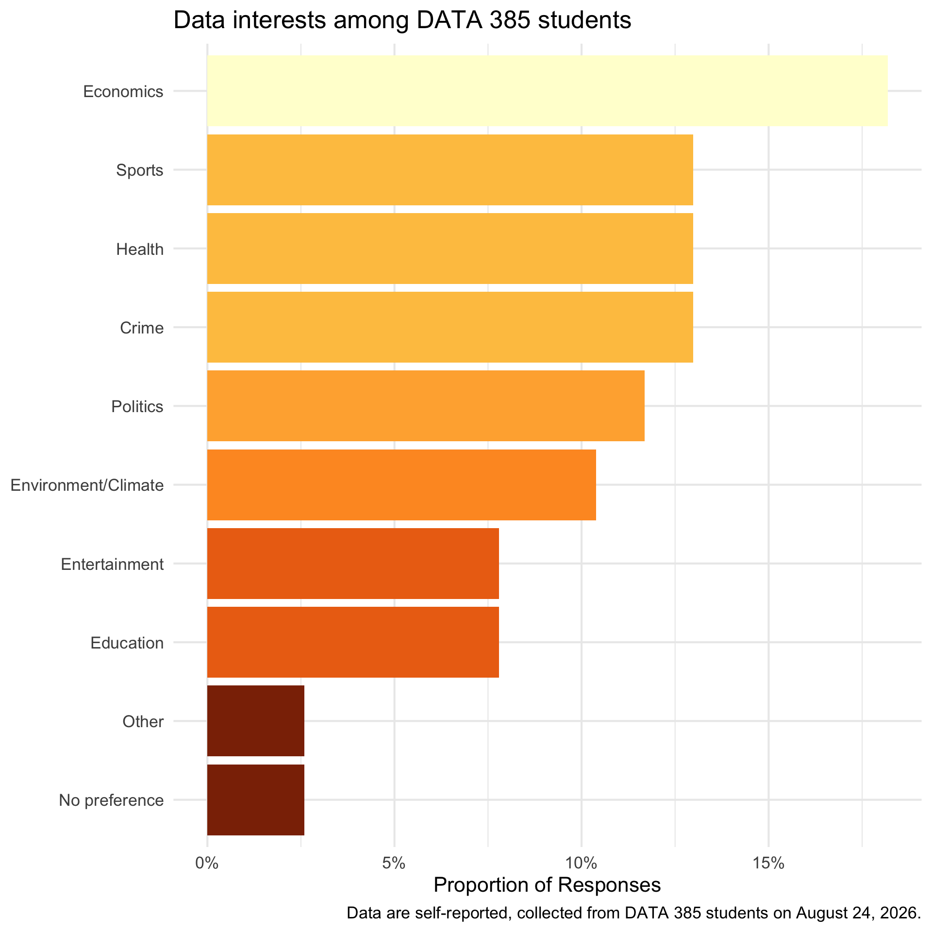
Visualize

Code
survey |>
   mutate(data_interests = str_remove_all(data_interests, "\\s*\\(.*?\\)|\\s*-\\s*")) |>
  separate_longer_delim(data_interests, delim = ",") |>
  mutate(data_interests = trimws(data_interests)) |>
  count(data_interests, sort = TRUE) |>
  mutate(prop = n / sum(n)) |>
  filter(!is.na(data_interests)) |>
  ggplot(aes(y = fct_reorder(data_interests, prop), x = prop, fill = prop)) +
  geom_col(show.legend = FALSE) +
  scale_y_discrete(labels = label_wrap(20)) +
  scale_x_continuous(labels = percent_format(accuracy = 1)) +
  scale_fill_distiller(palette = "YlOrBr") +
  labs(
    title = "Data interests among DATA 385 students",
    y = NULL,
    x = "Proportion of Responses",
    caption = "Data are self-reported, collected from DATA 385 students on August 24, 2026."
  ) +
  theme_minimal(base_size = 16)

Quantitative Numeric data

Tip

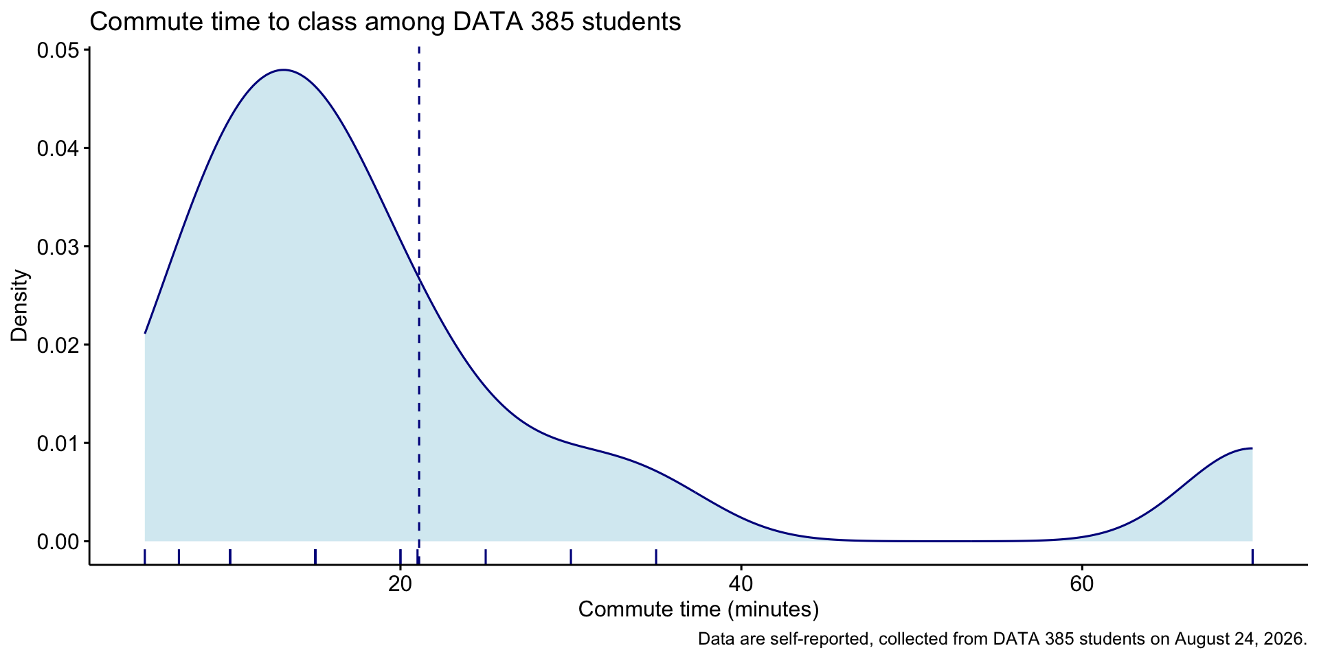
How long does it take you to commute from home to this classroom in minutes?

Code
survey |>
  ggdensity(
    x = "commute_minutes",
    fill = "lightblue",
    color = "darkblue",
    add_density = TRUE,
    add = "mean",
    rug = TRUE,
    title = "Commute time to class among DATA 385 students",
    xlab = "Commute time (minutes)",
    ylab = "Density"
  ) +
  labs(caption = "Data are self-reported, collected from DATA 385 students on August 24, 2026.")

Open ended text data

Tip

How do you learn best?

Code
survey |>
  select(learn_best)
# A tibble: 21 × 1
   learn_best                                                         
   <chr>                                                              
 1 Engaging lectures                                                  
 2 In person classes and lectures                                     
 3 Handwriting notes, working on code as a class, and lots of example…
 4 Personally, with live lectures where the professor uses the whiteb…
 5 Thoughtful and easy-to-follow lectures that I can refer back to if…
 6 Listening and watching examples then trying on my own.             
 7 Hands on/ trying things myself                                     
 8 Videos/Visual aids                                                 
 9 By practicing independently                                        
10 By doing                                                           
# ℹ 11 more rows

Tidy + Transform + Summarize

We can use text mining techniques, like tokenizing to words to explore this open-ended question:

Code
survey |>
  select(learn_best) |>
  unnest_tokens(word, learn_best) |>
  anti_join(stop_words, by = "word") |>
  count(word, sort = TRUE) |>
  filter(n > 2) |>
  print(n = Inf)
# A tibble: 4 × 2
  word         n
  <chr>    <int>
1 examples     4
2 lectures     4
3 learn        3
4 practice     3

We can also tokenize to bigrams (pairs of words):

Code
survey |>
  select(learn_best) |>
  tidytext::unnest_tokens(bigrams, learn_best, token = "ngrams", n = 2) |>
  count(bigrams, sort = TRUE) |>
  filter(n > 2) |>
  print(n = Inf)
# A tibble: 2 × 2
  bigrams      n
  <chr>    <int>
1 by doing     4
2 my own       3

Tidy + Transform + Visualize: Word cloud

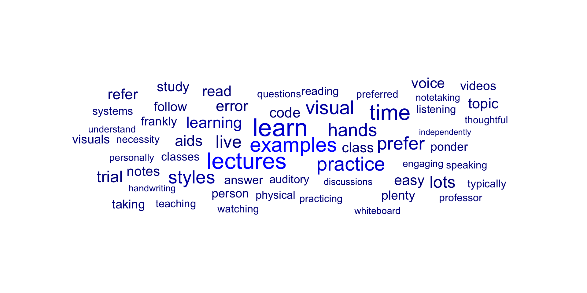
We can see the most frequently used words using a word cloud. Further tidying could be to remove words like “learn” and “lots” to remove “noise”

Code
survey |>
  select(learn_best) |>
  unnest_tokens(word, learn_best) |>
  anti_join(stop_words, by = "word") |>
  count(word, sort = TRUE) |>
  ggplot(aes(label = word, size = n, color = n)) +
  ggwordcloud::geom_text_wordcloud_area(shape = "square", 
                                        rm_outside=TRUE) +
  scale_color_gradient(low = "darkblue", high = "blue") + 
  scale_size_area(max_size = 24) +
  theme_minimal(base_size = 16) 

Mappable data

Tip

What is the zipcode of your hometown?

If you are from out of country, please enter 00000.

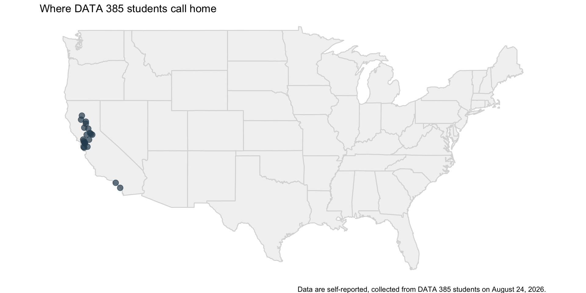
Tidy + Transform + Visualize: Map

Code
survey_locations <- survey |>
  mutate(zipcode = str_pad(zipcode, width = 5, side = "left", pad = "0")) |>
  left_join(zip_code_db, by = "zipcode")

survey_locations |>
  filter(!is.na(lat), zipcode != "00000") |>
  ggplot(aes(x = lng, y = lat)) +
  borders("state", colour = "gray85", fill = "gray95") +
  geom_point(color = "#2C4A5E", size = 3, alpha = 0.7) +
  coord_quickmap() +
  theme_void() +
  labs(
    title = "Where DATA 385 students call home",
    caption = "Data are self-reported, collected from DATA 385 students on August 24, 2026."
  )

Note: rows with zipcode 00000 (international students) are excluded from the map — worth calling out as a group separately rather than silently dropping them.

Longer answer write ins

Tip

If you’ve programmed before, which languages have you used, and how comfortable do you feel with each? If you haven’t programmed before, please leave this question blank.

Take a peek

And the answers are non-trivial to tidy up, e.g.,

Code
survey |>
  select(programming_language)
# A tibble: 21 × 1
   programming_language                                               
   <chr>                                                              
 1 C/C++ (very comfortable), Python (somewhat comfortable), R (somewh…
 2 C++, Java, Python                                                  
 3 Python - A little comfortable, R - A little comfortable, C++ - Som…
 4 mainly c++ and sql                                                 
 5 C/C++ (Comfortable), Python (Fairly Comfortable), Rust (Somewhat C…
 6 C++ (rusty but comfortable), Java (same),  PeopleCode (job related…
 7 R, C#                                                              
 8 C++, Python, Bash                                                  
 9 R studio: I’m not afraid of R, I think there is so much you can do…
10 C, C++, Java, Javascript, Typescript, Python, Go, Rust - very comf…
# ℹ 11 more rows

Can AI help make sense of this??

Prompt:

Summarize the following responses to the question “If you’ve programmed before, which languages have you used, and how comfortable do you feel with each? If you haven’t programmed before, please leave this question blank.”. Write your response in a short paragraph.

Response:

Most respondents have programming experience, with C/C++ by far the most common and generally the language people feel most comfortable using. Python, R, SQL, Java, Go, and Rust also appear frequently, though comfort levels vary from minimal or “rusty” to very comfortable. A few respondents mentioned additional experience with Bash, JavaScript/TypeScript, Assembly, C#, PeopleCode, HTML, and Unreal Engine Blueprints.

Can it be trusted 100%?

While models are getting better every day, they can be misleading, inaccurate, hallucinate or in general sound more confident than they are.

To get the best use out AI as a code helper, you have to have a reasonable level of understanding already to detect the inefficiencies, the omissions, the unnecessary stuff and frankly the bullshit. We are the keepers of the guardrails - and that position should be taken seriously.

Example of unnecessary / inefficiencies

I want to display a date “2026-08-25” as “Tue 8/25”

What Chat GPT gave me:

d <- d |> 
  mutate(
    date = paste0(
      format(date, "%a"), " ",
        as.integer(format(date, "%m")), "/",
        as.integer(format(date, "%d"))
      )
    )

What would also work

date = format(d$date, "%a %m/%d")

Course overview / How to get started

So how are we going to work together to teach you the skills that pay the bills?